Contents
Plot figures from experimental dataset for the publication:
Rindal, O. M. H., Rodriguez-Molares, A., & Austeng, A. (2017). The Dark Region Artifact in Adaptive Ultrasound Beamforming. IEEE International Ultrasonics Symposium, IUS, 1-4.
clear all;close all

% data location
url='http://ustb.no/datasets/';      % if not found downloaded from here
local_path = [ustb_path(),'/data/']; % location of example data

% Choose dataset
filename='beamformed_experimental_data.uff';

% check if the file is available in the local path or downloads otherwise
tools.download(filename, url, local_path);

% Read the beamformed images from the dataset
b_data_das = uff.read_object([local_path filename],'/b_data_das');
b_data_mv = uff.read_object([local_path filename],'/b_data_mv');
b_data_ebmv = uff.read_object([local_path filename],'/b_data_ebmv');
b_data_cf = uff.read_object([local_path filename],'/b_data_cf');
b_data_gcf = uff.read_object([local_path filename],'/b_data_gcf');
b_data_pcf = uff.read_object([local_path filename],'/b_data_pcf');
b_data_dmas = uff.read_object([local_path filename],'/b_data_dmas');
UFF: reading b_data_das [uff.beamformed_data]
UFF: reading b_data_mv [uff.beamformed_data]
UFF: reading b_data_ebmv [uff.beamformed_data]
UFF: reading b_data_cf [uff.beamformed_data]
UFF: reading b_data_gcf [uff.beamformed_data]
UFF: reading b_data_pcf [uff.beamformed_data]
UFF: reading b_data_dmas [uff.beamformed_data]
Let's write out some info about the authorship of this dataset
b_data_das.print_authorship
Name: 		 Beamformed dataset used to create the figures in
		 the publications under reference.
Reference: 	 Rindal, O. M. H., Rodriguez-Molares, A., &
		 Austeng, A. (2017). The Dark Region Artifact in
		 Adaptive Ultrasound Beamforming. IEEE
		 International Ultrasonics Symposium, IUS, 1-4.
Author(s): 	 Ole Marius Hoel Rindal <olemarius@olemarius.net>
Version: 	 1.0.0
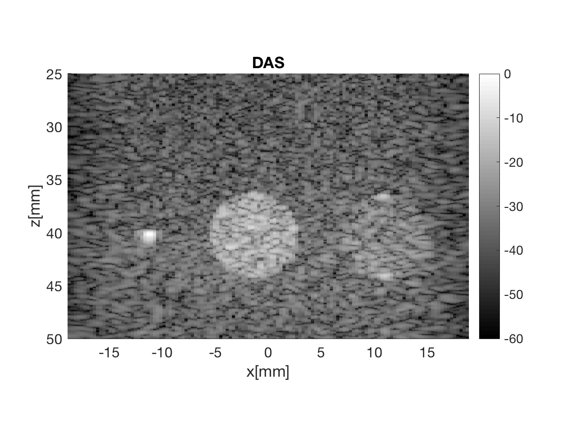
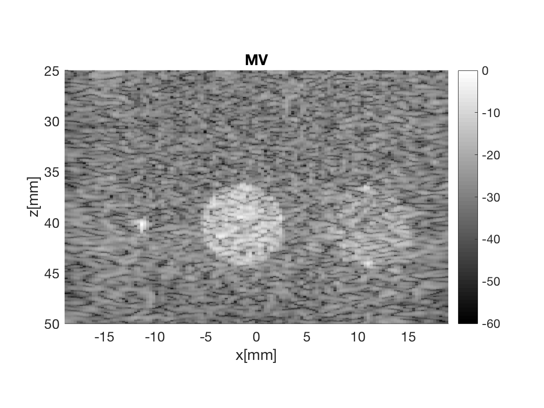
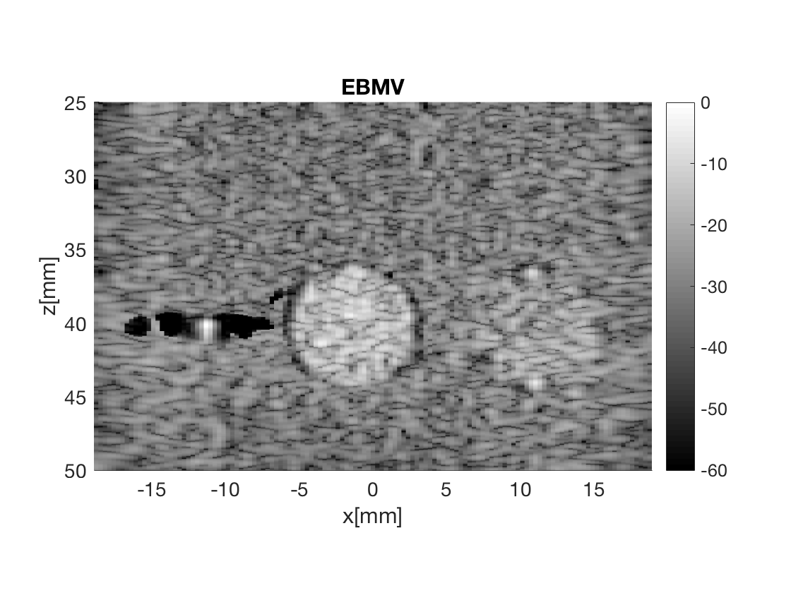
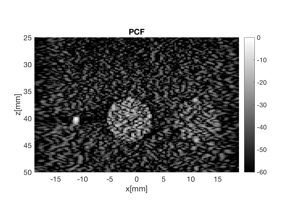
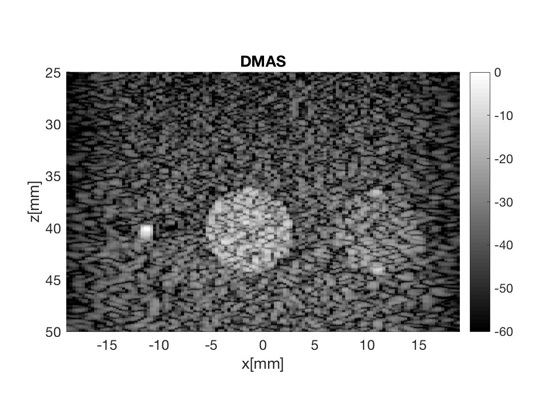
Display the images in Fig. 3
Massage the images into a cell array for easier processing in helper functions. Also display all images used in Fig. 3 in the publication.
image.all{1} = b_data_das.get_image();
image.tags{1} = 'DAS';
b_data_das.plot(1,'DAS');
image.all{2} = b_data_mv.get_image();
image.tags{2} = 'MV';
b_data_mv.plot(2,'MV');
image.all{3} = b_data_ebmv.get_image();
image.tags{3} = 'EBMV';
b_data_ebmv.plot(3,'EBMV');
image.all{4} = b_data_cf.get_image();
image.tags{4} = 'CF';
b_data_cf.plot(4,'CF');
image.all{5} = b_data_gcf.get_image();
image.tags{5} = 'GCF';
b_data_gcf.plot(5,'GCF');
image.all{6} = b_data_pcf.get_image();
image.tags{6} = 'PCF';
b_data_pcf.plot(6,'PCF');
image.all{7} = b_data_dmas.get_image();
image.tags{7} = 'DMAS';
b_data_dmas.plot(7,'DMAS');


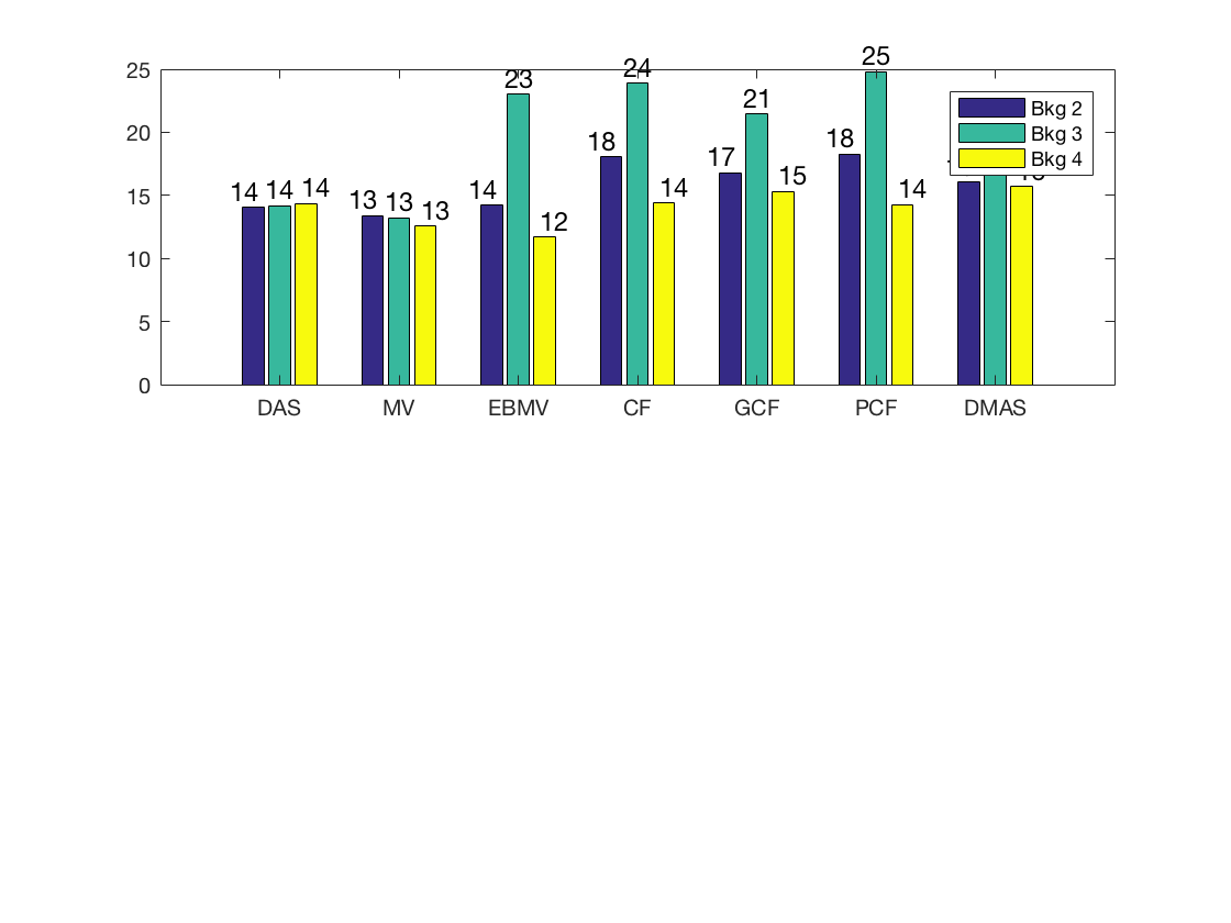
Measure the contrast creating Fig. 4
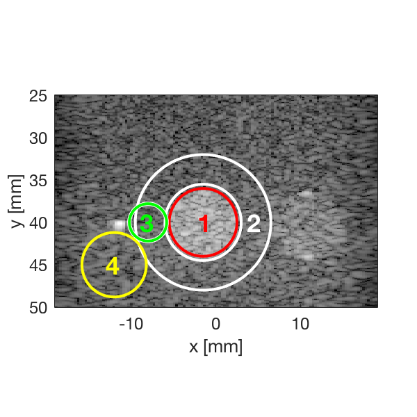
Measure the contrast of the different images creating Fig. 4 in the publication with the function measure_contrast_experimental_dra, also create the DAS image for Fig. 3 with regions indicated.
[CR,CR_alt,CR_alt_2,handle_DAS] = measure_contrast_experimental_dra...
                            (b_data_das,image,-1.5,40,4,4.5,8,-12,45,2.2,-8,40,3.8);

% Create bar plot for Fig. 4 in the publication.
[handle] = plot_contrast_differences_DRA(CR,CR_alt_2,CR_alt,image,'Bkg 2','Bkg 3','Bkg 4');
f12= figure(12);clf
set(f12,'Position',[100, 100, 550, 470]);
ax = subplot(2,1,1);
copyobj(allchild(handle),ax)
set(gca,'XTick',linspace(1,length(image.tags),length(image.tags)))
set(gca,'XTickLabel',image.tags)
ylabel('CR [dB]');
h_legend = legend('show','Location','best');
grid on
ylim([0 30]);
set(gca,'FontSize',12);
set(h_legend,'Position',[0.1525    0.7997    0.1209    0.1257]);