Contents
- Plot figures from simulated dataset for the publication:
- Let's write out some info about the authorship of this dataset
- Display the images in Fig. 1
- Measure the contrast creating Fig. 2
- Create a "data_cube" containing the wave field for each pixel.
- Plot the delayed wavefield in Fig. 5
- Plot the delayed wavefield in Fig. 6
Plot figures from simulated dataset for the publication:
Rindal, O. M. H., Rodriguez-Molares, A., & Austeng, A. (2017). The Dark Region Artifact in Adaptive Ultrasound Beamforming. IEEE International Ultrasonics Symposium, IUS, 1-4.
This script is available under /publications/IUS2017/Rindal_et_al_TheDarkRegionArtifactInAdaptiveUltrasoundBeamforming in the USTB repository.
clear all;close all

% data location
url='http://ustb.no/datasets/';      % if not found downloaded from here
local_path = [ustb_path(),'/data/']; % location of example data

% Choose dataset
filename='beamformed_simulated_data.uff';

% check if the file is available in the local path or downloads otherwise
tools.download(filename, url, local_path);

% Read the beamformed images from the dataset
b_data_das = uff.read_object([local_path filename],'/b_data_das');
b_data_mv = uff.read_object([local_path filename],'/b_data_mv');
b_data_ebmv = uff.read_object([local_path filename],'/b_data_ebmv');
b_data_cf = uff.read_object([local_path filename],'/b_data_cf');
b_data_gcf = uff.read_object([local_path filename],'/b_data_gcf');
b_data_pcf = uff.read_object([local_path filename],'/b_data_pcf');
b_data_dmas = uff.read_object([local_path filename],'/b_data_dmas');
b_data_tx = uff.read_object([local_path filename],'/b_data_tx');
UFF: reading b_data_das [uff.beamformed_data]
UFF: reading b_data_mv [uff.beamformed_data]
UFF: reading b_data_ebmv [uff.beamformed_data]
UFF: reading b_data_cf [uff.beamformed_data]
UFF: reading b_data_gcf [uff.beamformed_data]
UFF: reading b_data_pcf [uff.beamformed_data]
UFF: reading b_data_dmas [uff.beamformed_data]
UFF: reading b_data_tx [uff.beamformed_data]
UFF: reading sequence [uff.wave] [====================] 100%
Let's write out some info about the authorship of this dataset
b_data_das.print_authorship
Name: 		 Beamformed dataset used to create the figures in
		 the publications under reference.
Reference: 	 Rindal, O. M. H., Rodriguez-Molares, A., &
		 Austeng, A. (2017). The Dark Region Artifact in
		 Adaptive Ultrasound Beamforming. IEEE
		 International Ultrasonics Symposium, IUS, 1-4.
Author(s): 	 Ole Marius Hoel Rindal <olemarius@olemarius.net>
Version: 	 1.0.0
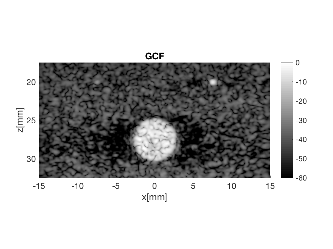
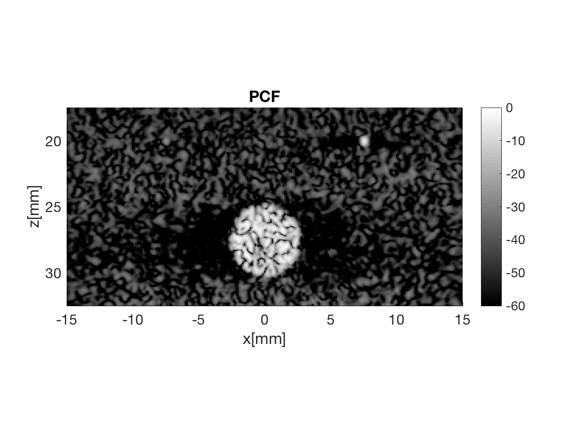
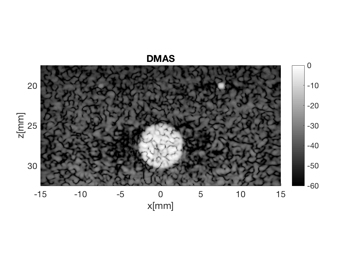
Display the images in Fig. 1
Massage the images into a cell array for easier processing in helper functions. Also display all images used in Fig. 1 in the publication.
image.all{1} = b_data_das.get_image();
image.tags{1} = 'DAS';
b_data_das.plot(1,'DAS');
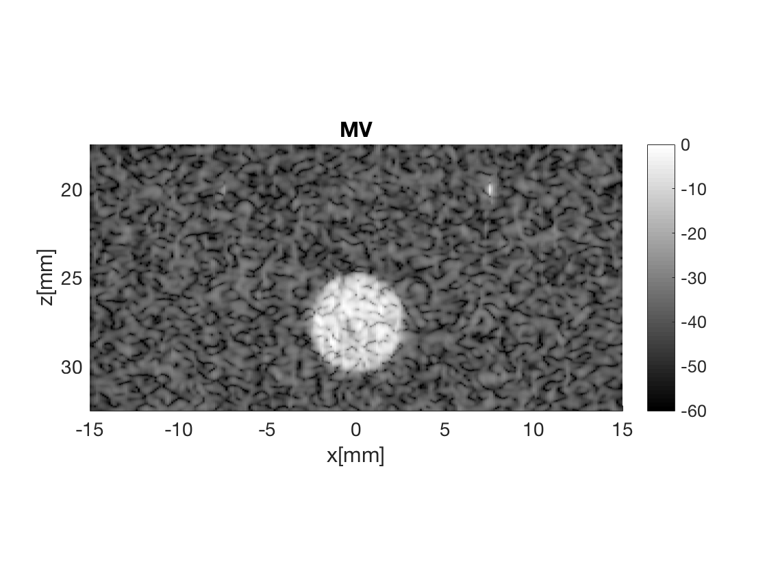
image.all{2} = b_data_mv.get_image();
image.tags{2} = 'MV';
b_data_mv.plot(2,'MV');
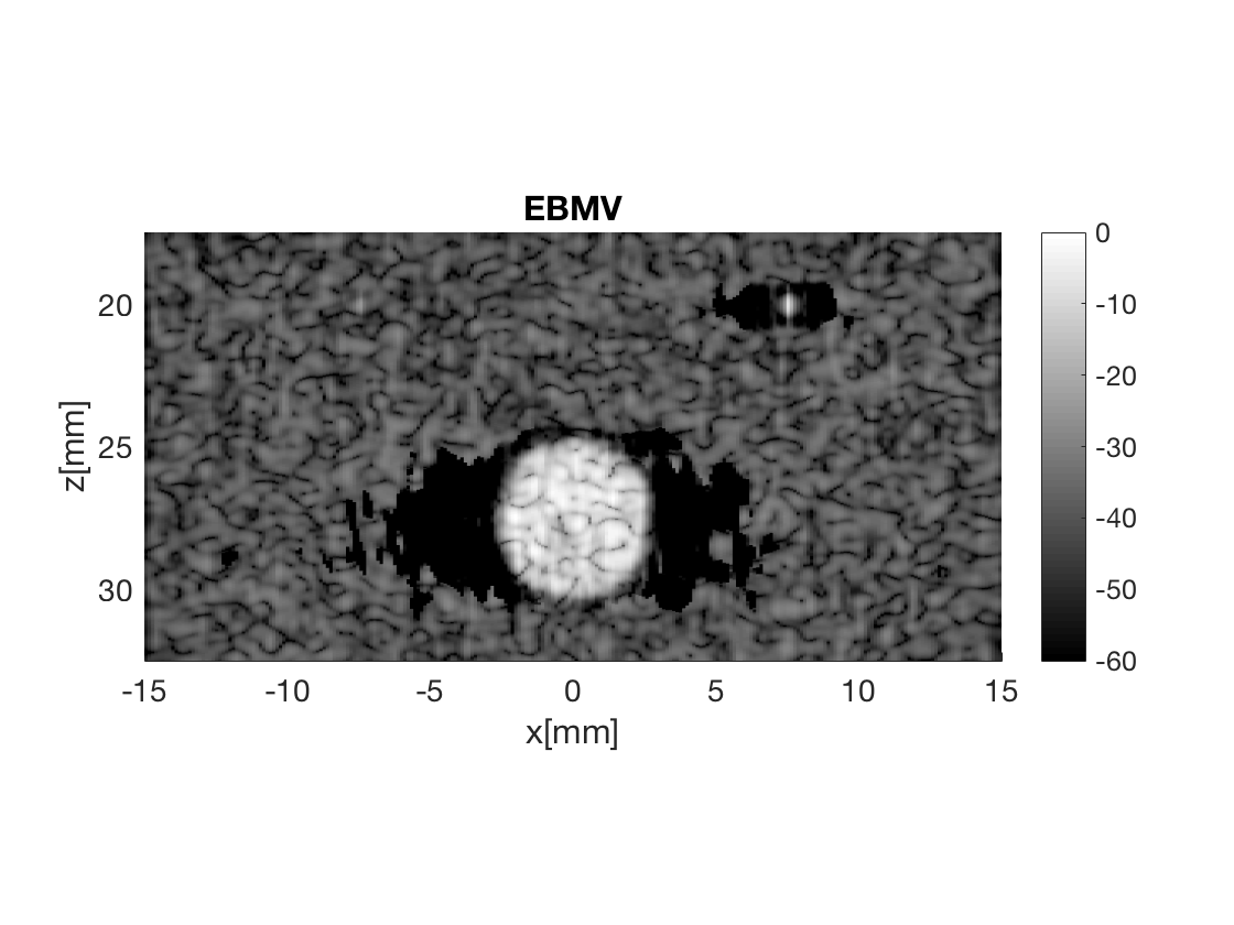
image.all{3} = b_data_ebmv.get_image();
image.tags{3} = 'EBMV';
b_data_ebmv.plot(3,'EBMV');
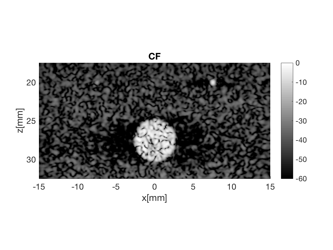
image.all{4} = b_data_cf.get_image();
image.tags{4} = 'CF';
b_data_cf.plot(4,'CF');
image.all{5} = b_data_gcf.get_image();
image.tags{5} = 'GCF';
b_data_gcf.plot(5,'GCF');
image.all{6} = b_data_pcf.get_image();
image.tags{6} = 'PCF';
b_data_pcf.plot(6,'PCF');
image.all{7} = b_data_dmas.get_image();
image.tags{7} = 'DMAS';
b_data_dmas.plot(7,'DMAS');

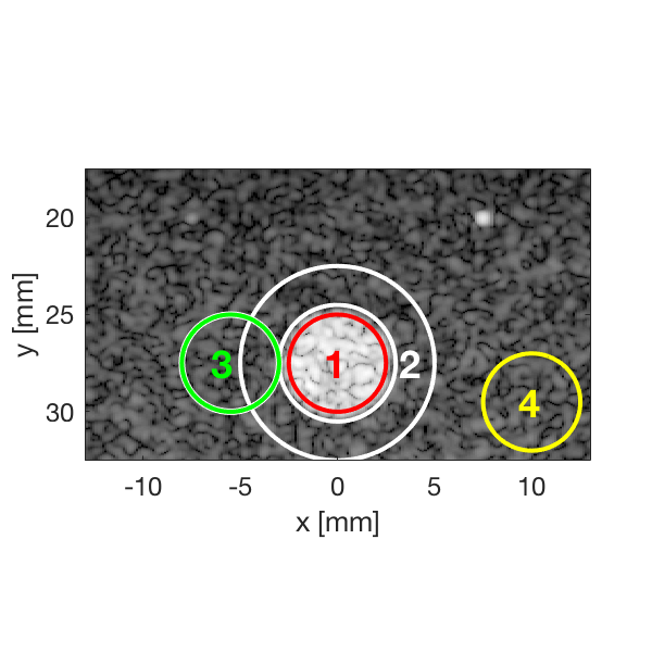
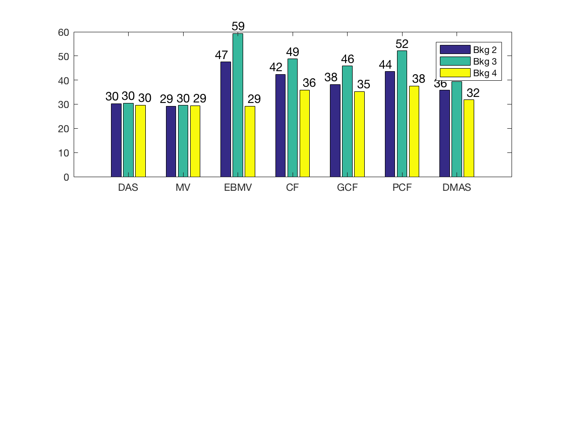
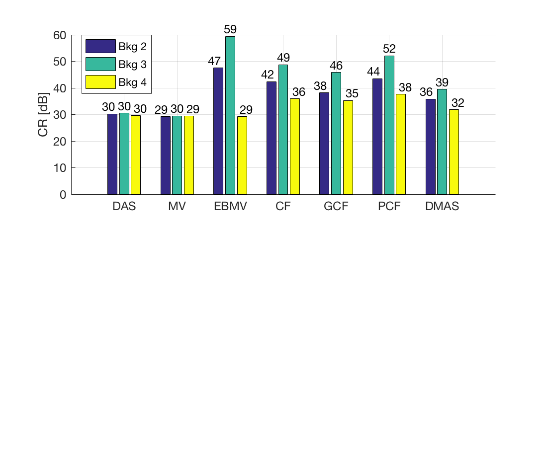
Measure the contrast creating Fig. 2
Measure the contrast of the different images creating Fig. 2 in the publication with the function measure_contrast_experimental_dra, also create the DAS image for Fig. 1 with regions indicated.
[CR,CR_alt,CR_alt_2,handle_DAS] = measure_contrast_simulated_dra...
                                   (b_data_tx,image,0,27.5,2.5,3,5,10,29.5,2.5,-5.5,27.5);

[handle] = plot_contrast_differences_DRA(CR,CR_alt_2,CR_alt,image,'Bkg 2','Bkg 3','Bkg 4');
f12= figure(12);clf
set(f12,'Position',[100, 100, 550, 470]);
ax = subplot(2,1,1);
copyobj(allchild(handle),ax)
set(gca,'XTick',linspace(1,length(image.tags),length(image.tags)))
set(gca,'XTickLabel',image.tags)
ylabel('CR [dB]');
h_legend = legend('show','Location','best');
grid on
ylim([0 60]);
set(gca,'FontSize',12);
set(h_legend,'Position',[0.1525    0.7997    0.1209    0.1257])
Create a "data_cube" containing the wave field for each pixel.
To plot the delayed wave field of the received channel data we need to reshape the b_data_tx beamformed_data which consist of the STAI channel data delayed with each transmit sequence summed.
data_cube = reshape(b_data_tx.data,b_data_tx.scan.N_z_axis,...
                                b_data_tx.scan.N_x_axis,b_data_tx.N_channels);
% Let's normalize it to the maximum
data_cube = data_cube./max(data_cube(:));
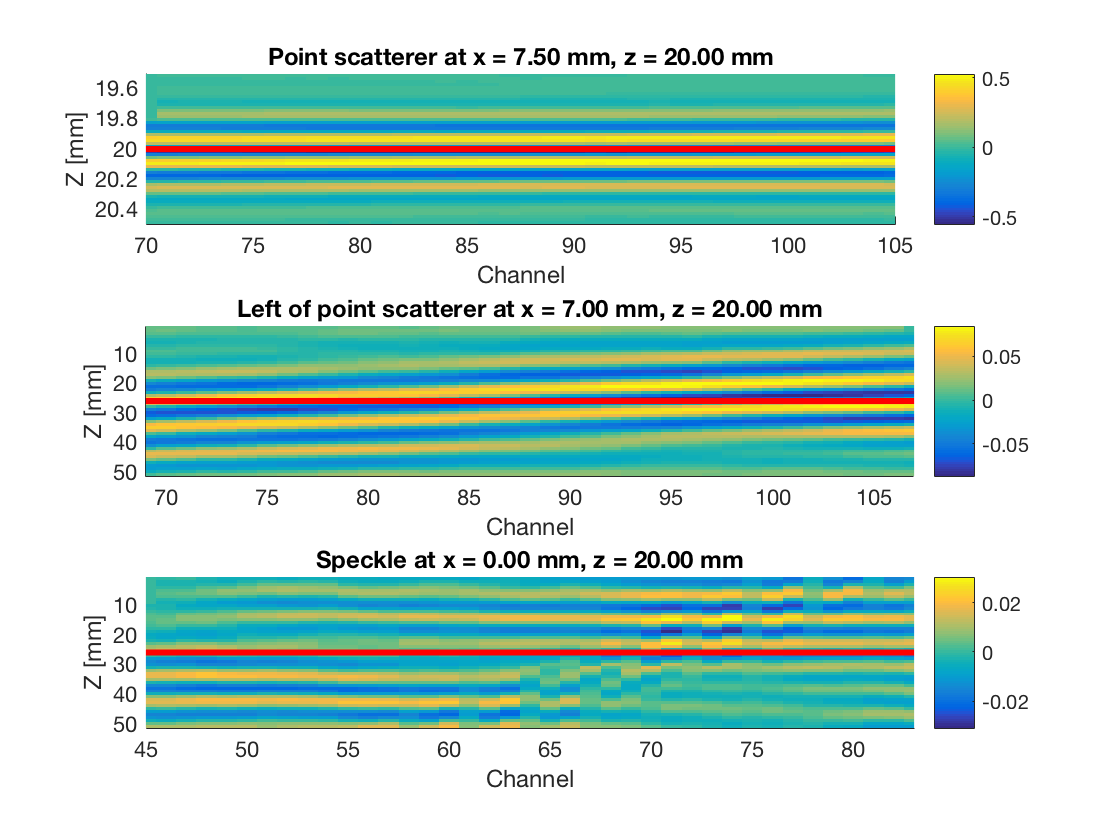
Plot the delayed wavefield in Fig. 5
The delayed wavefield from the point scatterer at x = 7.5 mm and z = 20 mm, to the left of the point at z = 7 mm and the speckle at x = 0 mm.
z_pixel_pos = 20e-3;
x_pixel_pos_point = 7.5e-3;
x_pixel_pos_left_of_point = 7e-3;
x_pixel_pos_speckle = 0e-3;

z_spacing = 25;

[~,z_idx] = min(abs(b_data_tx.scan.z_axis-z_pixel_pos));
[~,x_idx_point] = min(abs(b_data_tx.scan.x_axis-x_pixel_pos_point));
[~,x_idx_left_of_point] = min(abs(b_data_tx.scan.x_axis-x_pixel_pos_left_of_point));
[~,x_idx_speckle] = min(abs(b_data_tx.scan.x_axis-x_pixel_pos_speckle));

f100 = figure(100);clf
subplot(311); hold on
imagesc(1:b_data_tx.N_channels,b_data_tx.scan.z_axis(z_idx-z_spacing:z_idx+z_spacing)*10^3,...
                    real(squeeze(data_cube(z_idx-z_spacing:z_idx+z_spacing,x_idx_point,:))));
plot([65 115],[b_data_tx.scan.z_axis(z_idx)*10^3 b_data_tx.scan.z_axis(z_idx)*10^3],...
                                                            'linewidth',3,'color',[1,0,0]);
set(gca,'Ydir','reverse')
axis tight
colorbar
xlim([70 105]);
xlabel('Channel');ylabel('Z [mm]');
set(gca,'FontSize',11);
title(sprintf('Point scatterer at x = %.2f mm, z = %.2f mm',x_pixel_pos_point*10^3,z_pixel_pos*10^3));

subplot(312);hold on
imagesc(real(squeeze(data_cube(z_idx-z_spacing:z_idx+z_spacing,x_idx_left_of_point,:))));
plot([65 110],[z_spacing+1 z_spacing+1],'linewidth',3,'color',[1,0,0])
set(gca,'Ydir','reverse')
axis tight
xlim([69 107]);
colorbar
xlabel('Channel');ylabel('Z [mm]');
set(gca,'FontSize',11);
title(sprintf('Left of point scatterer at x = %.2f mm, z = %.2f mm',x_pixel_pos_left_of_point*10^3,...
                                                                              z_pixel_pos*10^3));

subplot(313);hold on
imagesc(real(squeeze(data_cube(z_idx-z_spacing:z_idx+z_spacing,x_idx_speckle,:))));
plot([0 128],[z_spacing+1 z_spacing+1],'linewidth',3,'color',[1,0,0])
set(gca,'Ydir','reverse')
axis tight
xlim([45 83]);
colorbar
xlabel('Channel');ylabel('Z [mm]');
set(gca,'FontSize',11);
title(sprintf('Speckle at x = %.2f mm, z = %.2f mm',x_pixel_pos_speckle*10^3,z_pixel_pos*10^3));
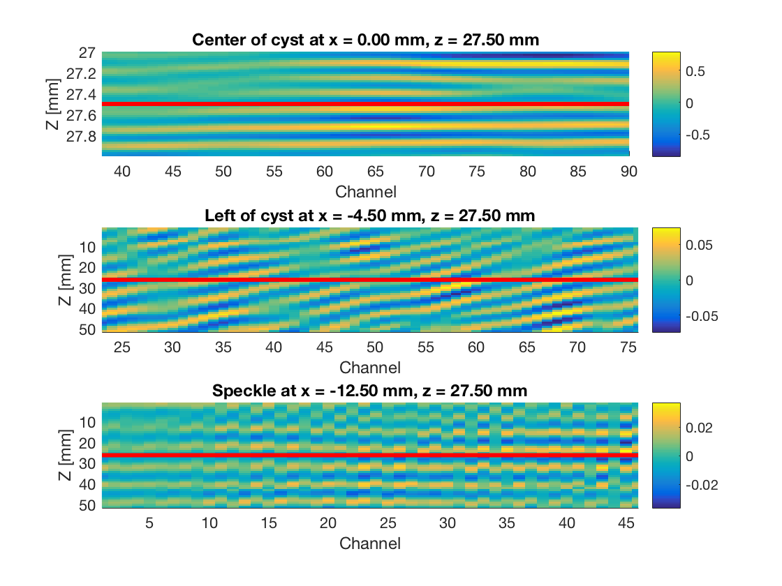
Plot the delayed wavefield in Fig. 6
The delayed wavefield from the cyst at x = 0 mm and z = 27.5 mm, to the left of the cyst at z = -4.5 mm and the speckle at x = -12.5 mm.
z_pixel_pos = 27.5e-3;
x_pixel_pos_point = 0e-3;
x_pixel_pos_left_of_point = -4.5e-3;
x_pixel_pos_speckle = -12.5e-3;

z_spacing = 25;

[~,z_idx] = min(abs(b_data_tx.scan.z_axis-z_pixel_pos));
[~,x_idx_point] = min(abs(b_data_tx.scan.x_axis-x_pixel_pos_point));
[~,x_idx_left_of_point] = min(abs(b_data_tx.scan.x_axis-x_pixel_pos_left_of_point));
[~,x_idx_speckle] = min(abs(b_data_tx.scan.x_axis-x_pixel_pos_speckle));

f101 = figure(101);clf
subplot(311); hold on
imagesc(1:b_data_tx.N_channels,b_data_tx.scan.z_axis(z_idx-z_spacing:z_idx+z_spacing)*10^3,...
                           real(squeeze(data_cube(z_idx-z_spacing:z_idx+z_spacing,x_idx_point,:))));
plot([1 128],[b_data_tx.scan.z_axis(z_idx)*10^3 b_data_tx.scan.z_axis(z_idx)*10^3],...
                                                            'linewidth',3,'color',[1,0,0]);
set(gca,'Ydir','reverse')
axis tight
colorbar
xlim([38 90]);
xlabel('Channel');ylabel('Z [mm]');
set(gca,'FontSize',11);
title(sprintf('Center of cyst at x = %.2f mm, z = %.2f mm',x_pixel_pos_point*10^3,z_pixel_pos*10^3));

subplot(312);hold on
imagesc(real(squeeze(data_cube(z_idx-z_spacing:z_idx+z_spacing,x_idx_left_of_point,:))));
plot([1 128],[z_spacing+1 z_spacing+1],'linewidth',3,'color',[1,0,0])
set(gca,'Ydir','reverse')
axis tight
xlim([23 76]);
colorbar
xlabel('Channel');ylabel('Z [mm]');
set(gca,'FontSize',11);
title(sprintf('Left of cyst at x = %.2f mm, z = %.2f mm',...
                                            x_pixel_pos_left_of_point*10^3,z_pixel_pos*10^3));

subplot(313);hold on
imagesc(real(squeeze(data_cube(z_idx-z_spacing:z_idx+z_spacing,x_idx_speckle,:))));
plot([1 128],[z_spacing+1 z_spacing+1],'linewidth',3,'color',[1,0,0])
set(gca,'Ydir','reverse')
axis tight
xlim([1 46]);
colorbar
xlabel('Channel');ylabel('Z [mm]');
set(gca,'FontSize',11);
title(sprintf('Speckle at x = %.2f mm, z = %.2f mm',x_pixel_pos_speckle*10^3,z_pixel_pos*10^3));