FLUST example: Simulation of a spinning disk phantom

In this example, FLUST is used to simulate IQ Doppler signals from a spinning disk phantom, using unfocused ultrasound transmissions. This phantom represents a special case where the start and end of the flowlines are both at x = 0 in the lower part of the phantom, creating a discontinuity at this border.

DATA OUTPUT PARAMETERS
QUALITY PARAMETERS
PERFORMANCE PARAMETERS
DEFINE ACQUSITION SETUP / PSF FUNCTIONS
DEFINE PHANTOM FUNCTION
FLUST main loop
VISUALIZE FIRST REALIZATION using the built-in beamformed data object
True velocities
SAVE realizations and metadata

% Updated 27/02/2023,
% Joergen Avdal (jorgen.avdal@ntnu.no),
% Ingvild Kinn Ekroll (ingvild.k.ekroll@ntnu.no)

% If using FLUST for scientific publications, please cite the original paper
% Avdal et al: Fast Flow-Line-Based Analysis of Ultrasound Spectral and
% Vector Velocity Estimators, tUFFC, 2019. DOI: 10.1109/TUFFC.2018.2887398

% FLUST is a simulation tool based on flowlines, useful for producing many
% realizations of the same flowfield. The motivation for making FLUST was
% to faciliate accurate assessment of statistical properties of velocity
% estimators like bias and variance.

% Using FLUST requires the user to provide/select two functions, one to create
% the flowlines, and one to calculate the PSFs from a vector of spatial
% positions.

% After running this script, variable realTab contains realizations, and
% variables PSFs and PSFstruct contains point spread functions of the last flow line.

% FLUST accounts for interframe motion in plane wave sequences, assuming
% uniform firing rate, but not in scanned sequences.

% How to use FLUST:
% 1) Provide/select function to calculate PSFs from a vector of spatial positions.
% 2) Run FLUST on phantom of interest.
% 3) Apply your favorite velocity estimator to realizations.
% 4) Assess statistical properties of estimator, optimize estimator.
% 5) Publish results, report statistical properties, make results
%    reproducible, cite original paper DOI: 10.1109/TUFFC.2018.2887398


clear all;
close all;

setPathsScript;

DATA OUTPUT PARAMETERS

First, we define the firing rate of the simulated signal, the number of realizations and the ensemble size, and whether or not this is a simulation of contrast bubbles or not:


s = struct();

s.firing_rate = 12000; % firing rate of output signal, (Doppler PRF) = (firing rate)/(nr of firings)
s.nrReps = 10;         % nr of realizations
s.nrSamps = 40;       % nr of slow time samples in each realization (Ensemble size)

s.contrastMode = 0;      % is set to 1, will simulate contrast scatterers propagating in flow field
s.contrastDensity = 0.1; % if using contrastMode, determines the density of scatterers, typically < 0.2

QUALITY PARAMETERS

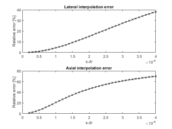
Then, a recommended distance for PSF function seedpoints is calculated based on a user defined accepted value for interpolation error in percent:

s.interpErrorLimit = 4; % FLUST will set s.dr to attain interpolation error smaller than this value in percent

PERFORMANCE PARAMETERS

Choose whether or not to utilize your GPU, and how many scanlines/channels to process simultaneously when generating realizations from calculated PSFs. Optimal values depend primarily on GPU specifications and available memory.

s.chunksize = 16; % chunking on scanlines, adjust according to available memory.
s.useGPU = 1;

DEFINE ACQUISITION SETUP / PSF FUNCTIONS

Set desired PSF function and acquisition parameters. If not set, predefined values are used (see individual PSF function definitions). Chunksize here refers to the number of simultaneously processed PSFs.

s.PSF_function = @PSFfunc_LinearProbe_PlaneWaveImaging_txApod;

% Transducer and acquisition parameters. Print s.PSF_params after running simulation to see which parameters can be set.
s.PSF_params = [];

% Transducer params
s.PSF_params.trans.f0 = 12.0e6;
s.PSF_params.trans.pulse_duration = 1.5;
s.PSF_params.trans.element_height = 3e-3;
s.PSF_params.trans.lens_el = 0.01;
s.PSF_params.trans.pitch = 100e-6;
s.PSF_params.trans.kerf = 10e-6;
s.PSF_params.trans.N = 256;

% Acquisition params
s.PSF_params.acq.alphaTx = [0]*pi/180;
s.PSF_params.acq.alphaRx = [0]*pi/180;
s.PSF_params.acq.F_number = 1.0;
s.PSF_params.acq.tx_apod = 'none';

% Image/scan region params
s.PSF_params.scan.rx_apod = 'blackman';
s.PSF_params.scan.xStart = -5e-3;
s.PSF_params.scan.xEnd = 5e-3;
s.PSF_params.scan.Nx = 128;
s.PSF_params.scan.zStart = 5e-3;
s.PSF_params.scan.zEnd = 15e-3;
s.PSF_params.scan.Nz = 128;

% Runtime params
s.PSF_params.run.chunkSize = 125;

DEFINE PHANTOM FUNCTION

Set desired phantom and phantom parameters. If not set, predefined values are used (see individual phantom function definitions).

s.phantom_function = @Phantom_spinningDisk;

% Phantom parameters. Print s.phantom_params after running simulation to see which parameters can be set.
s.phantom_params = [];
s.phantom_params.maxVel = 0.7;
s.phantom_params.minVel = 0.2;
s.phantom_params.diameter = 0.007; %m
s.phantom_params.depth = 0.01;

% To output true velocities in phantom, define grid
myX = linspace(s.PSF_params.scan.xStart,s.PSF_params.scan.xEnd,s.PSF_params.scan.Nx);
myZ = linspace(s.PSF_params.scan.zStart,s.PSF_params.scan.zEnd,s.PSF_params.scan.Nz);
myY = 0;
[X,Z,Y] =  meshgrid(myX,myZ,myY);

% make phantom, get true velocity and phantom parameters
[flowField, s.phantom_params, GT] = s.phantom_function(s.phantom_params,X,Y,Z); % flowField should have timetab and postab fields

FLUST main loop

Run your FLUST simulation!

runFLUST;

Suggested upper limit for s.dr for axial interpolation 3e-05
Suggested upper limit for s.dr for lateral interpolation 9e-05
s.dr changed to 3e-05
Finished!

VISUALIZE FIRST REALIZATION using the built-in beamformed data object

firstRealization = realTab(:,:,:,1,1);

b_data = uff.beamformed_data();
b_data.scan = PSFstruct.scan;
b_data.data = reshape(firstRealization,size(firstRealization,1)*size(firstRealization,2),1,1,size(firstRealization,3));
b_data.frame_rate = 20;
b_data.plot([],'Flow from FLUST', 20);

True velocities

The true phantom velocities are available for visualization. Future versions of this example will provide a demonstration of how to use the built in velocity estimator performance assessment tools in FLUST.

 % GT_rsh = reshape( GT, [s.PSF_params.scan.Nz s.PSF_params.scan.Nx 1 3] ); 
 % figure(2); imagesc(X(:), Z(:), GT_rsh(:,:,1,1)); axis equal; 
 % title('Vx') % Example, looking at x component of velocity field 
 % figure(3); imagesc(X(:), Z(:), GT_rsh(:,:,1,3)); axis equal; 
 % title('Vz') % Example, looking at z component of velocity field

SAVE realizations and metadata

 % tag = 'myTag'; 
 % saveBinary( tag);