Contents

Focused Linear scan with L7-4 probe in Verasonics demonstrating RTB

This script is available in the USTB repository as /USTB/publications/IUS2018/Rindal_et_al_ASimpleArtifactFreeVirtualSourceModel/

This example demonstrates the RTB implementation and demonstrates different fixes to the artifact occuring near the focus.

One solution is the transmit delay model introduced in Nguyen, N. Q., & Prager, R. W. (2016). High-Resolution Ultrasound Imaging With Unified Pixel-Based Beamforming. IEEE Trans. Med. Imaging, 35(1), 98-108.

Another solution is a simpler model assuming PW around focus.

This scripts creates the figure used in the procedings paper

%Rindal, O. M. H., Rodriguez-Molares, A., Austeng, A. (2018). A simple, artifact-free,
% virtual source model. Ultrasonics Symposium (IUS), 2018 IEEE International, 1–4.
%
% _by Ole Marius Hoel Rindal <olemarius@olemarius.net> Last updated: 2018/10/05

Read channel data

clear all; close all;

% data location
url='http://ustb.no/datasets/';      % if not found downloaded from here

filename='L7_FI_IUS2018.uff';
tools.download(filename, url, data_path);
channel_data =uff.read_object([data_path filesep filename],'/channel_data');

UFF: reading channel_data [uff.channel_data]
UFF: reading sequence [uff.wave] [====================] 100%

Define Scan

x_axis=zeros(channel_data.N_waves,1);
for n=1:channel_data.N_waves
    x_axis(n)=channel_data.sequence(n).source.x;
end
z_axis=linspace(1e-3,62e-3,512*2).';
scan=uff.linear_scan('x_axis',x_axis,'z_axis',z_axis);

Conventional Scanline Beamforming

mid = midprocess.das();
mid.dimension = dimension.both();

mid.channel_data = channel_data;
mid.scan=scan;

mid.transmit_apodization.window=uff.window.scanline;

mid.receive_apodization.window=uff.window.none;
mid.receive_apodization.f_number=1.7;

b_data=mid.go();

USTB General beamformer MEX v1.1.2 .............done!

Display the Conventional Scanline Image

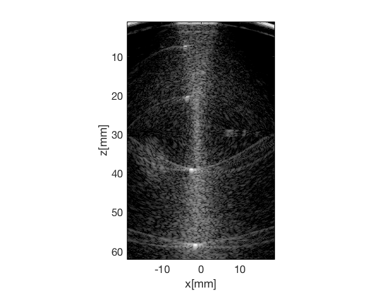
This creates the image for Fig. 3a and 4a.

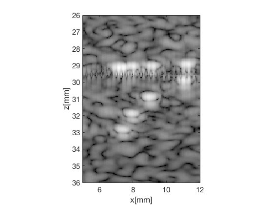
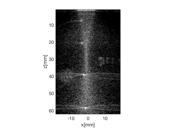
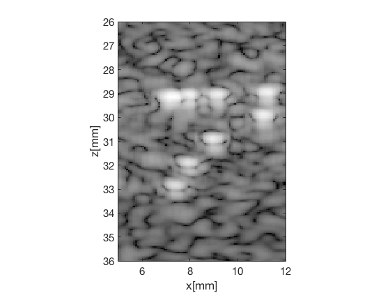
b_data.plot([],'Conventional one scanline per transmit');

f456 = figure(456);clf;
imagesc(scan.x_axis*1000,z_axis*1000,b_data.get_image);
colormap gray; caxis([-60 0]); axis image;
xlabel('x[mm]');ylabel('z[mm]');
set(gca,'Fontsize',15)
saveas(f456,[ustb_path,'/publications/IUS2018/Rindal_et_al_ASimpleArtifactFreeVirtualSourceModel/Figures/full_image_conventional.eps'],'eps2c')
axis([5 12 26 36])
saveas(f456,[ustb_path,'/publications/IUS2018/Rindal_et_al_ASimpleArtifactFreeVirtualSourceModel/Figures/full_image_conventional_zoomed.eps'],'eps2c')

Create scan with MLA's

MLA = 4;
scan_RTB=uff.linear_scan('x_axis',linspace(x_axis(1),x_axis(end),...
                                    length(x_axis)*MLA)','z_axis',z_axis);

Retrospective beamforming (RTB) with conventional spherical model

We firs set up the beamforming to create all the images created from each transmit.

mid_RTB_spherical_model=midprocess.das();
mid_RTB_spherical_model.dimension = dimension.receive();

mid_RTB_spherical_model.channel_data=channel_data;
mid_RTB_spherical_model.scan=scan_RTB;
mid_RTB_spherical_model.transmit_delay_model = transmit_delay_model.spherical;

mid_RTB_spherical_model.transmit_apodization.window=uff.window.none;
mid_RTB_spherical_model.transmit_apodization.f_number = 2;
mid_RTB_spherical_model.transmit_apodization.MLA = MLA;
mid_RTB_spherical_model.transmit_apodization.MLA_overlap = 1;
mid_RTB_spherical_model.transmit_apodization.minimum_aperture = [3.000e-03 3.000e-03];

mid_RTB_spherical_model.receive_apodization.window=uff.window.boxcar;
mid_RTB_spherical_model.receive_apodization.f_number=1.7;
b_data_RTB=mid_RTB_spherical_model.go();

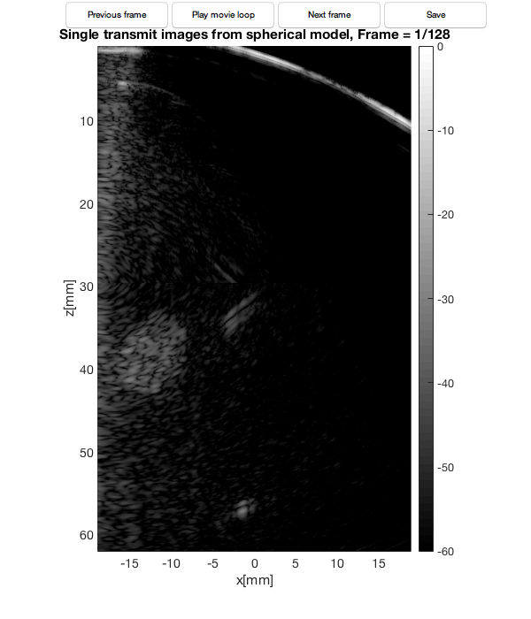
b_data_RTB.plot(767,'Single transmit images from spherical model')

USTB General beamformer MEX v1.1.2 .............done!

ans = 

  Figure (767) with properties:

      Number: 767
        Name: ''
       Color: [0.9400 0.9400 0.9400]
    Position: [100 100 600 700]
       Units: 'pixels'

  Use GET to show all properties

Show and save the individual transmit image from the convetional spherical model

This creates the image in Fig. 7a.

tx = 61;
f556 = figure(556);clf;
img = reshape(b_data_RTB.data,scan_RTB.N_z_axis,scan_RTB.N_x_axis,channel_data.N_waves);

imagesc(scan_RTB.x_axis*1000,z_axis*1000,db(abs(img(:,:,tx)./max(max(img(:,:,tx))))));
colormap gray; caxis([-60 0]); axis image;
xlabel('x[mm]');ylabel('z[mm]');
set(gca,'Fontsize',15)
saveas(f556,[ustb_path,'/publications/IUS2018/Rindal_et_al_ASimpleArtifactFreeVirtualSourceModel/Figures/full_image_vs_single_tx.eps'],'eps2c')

Adjust the beamforming to apply the tukey window on the individual transmit images

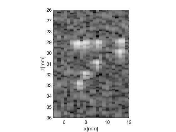
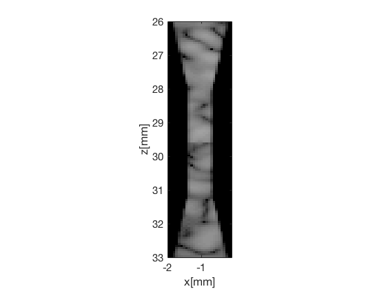
This creates the images in Fig. 8a.

mid_RTB_spherical_model.transmit_apodization.window=uff.window.tukey25;
b_data_RTB_weighted=mid_RTB_spherical_model.go();

f556 = figure(556);
img = reshape(b_data_RTB_weighted.data,scan_RTB.N_z_axis,scan_RTB.N_x_axis,channel_data.N_waves);
imagesc(scan_RTB.x_axis*1000,z_axis*1000,db(abs(img(:,:,tx)./max(max(img(:,:,tx))))));
colormap gray; caxis([-60 0]); axis image;
xlabel('x[mm]');ylabel('z[mm]');
set(gca,'Fontsize',15)
axis([-2 -0.1 26 33])
saveas(f556,[ustb_path,'/publications/IUS2018/Rindal_et_al_ASimpleArtifactFreeVirtualSourceModel/Figures/vs_zoomed_single_tx.eps'],'eps2c')

uff.apodization: Inputs and outputs are unchanged. Skipping process.
USTB General beamformer MEX v1.1.2 .............done!

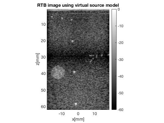
Adjust the beamforming to create the full RTB image from the spherical model

mid_RTB_spherical_model.dimension = dimension.both();
mid_RTB_spherical_model.transmit_apodization.window=uff.window.tukey25;
b_data_RTB=mid_RTB_spherical_model.go();

b_data_RTB.plot(768,'RTB image using virtual source model');

% We need to compensate with the TX transmit apodization as weighting to
% get a more uniform image
% Calculate the transmit apodzation used to compensate image
tx_apod = mid_RTB_spherical_model.transmit_apodization.data;

b_data_RTB_weighted = uff.beamformed_data(b_data_RTB);
b_data_RTB_weighted.data = b_data_RTB_weighted.data.*(1./sum(tx_apod,2));
b_data_RTB_weighted.plot(10,'RTB image using virtual source model, TX weighted');

uff.apodization: Inputs and outputs are unchanged. Skipping process.
uff.apodization: Inputs and outputs are unchanged. Skipping process.
USTB General beamformer MEX v1.1.2 .............done!
uff.apodization: Inputs and outputs are unchanged. Skipping process.

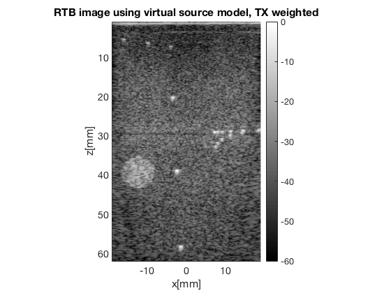
After compensating with TX transmit apodization as weighting we get the final image shown in Fig. 3b and 4b.

f456 = figure(456)
imagesc(scan_RTB.x_axis*1000,z_axis*1000,b_data_RTB_weighted.get_image);
colormap gray; caxis([-60 0]); axis image;
xlabel('x[mm]');ylabel('z[mm]');
set(gca,'Fontsize',15)
saveas(f456,[ustb_path,'/publications/IUS2018/Rindal_et_al_ASimpleArtifactFreeVirtualSourceModel/Figures/full_image_vs.eps'],'eps2c')
axis([5 12 26 36])
saveas(f456,[ustb_path,'/publications/IUS2018/Rindal_et_al_ASimpleArtifactFreeVirtualSourceModel/Figures/full_image_vs_zoomed.eps'],'eps2c')

f456 = 

  Figure (456) with properties:

      Number: 456
        Name: ''
       Color: [0.9400 0.9400 0.9400]
    Position: [440 378 560 420]
       Units: 'pixels'

  Use GET to show all properties

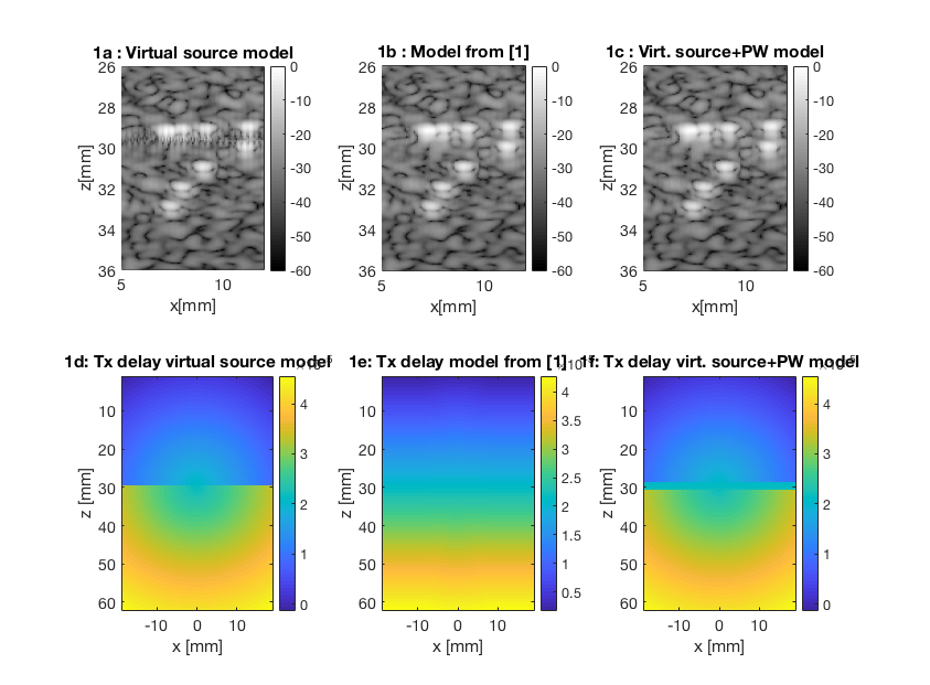
Notice the line/articat along 29.6 mm, the transmit focus, which is the artifact we aim at getting rid of :)

RTB using Nguyen & Prager's unified transmit model

beamforming using the "unified pixelbased beamforming" model from Nguyen, N. Q., & Prager, R. W. (2016). High-Resolution Ultrasound Imaging With Unified Pixel-Based Beamforming. IEEE Trans. Med. Imaging, 35(1), 98-108. We firs set up the beamforming to create all the images created from each transmit.

mid_RTB_unified_model =midprocess.das();
mid_RTB_unified_model.dimension = dimension.receive();

mid_RTB_unified_model.channel_data=channel_data;
mid_RTB_unified_model.scan=scan_RTB;
mid_RTB_unified_model.transmit_delay_model = transmit_delay_model.unified;

mid_RTB_unified_model.transmit_apodization.window=uff.window.none;
mid_RTB_unified_model.transmit_apodization.f_number = 2;
mid_RTB_unified_model.transmit_apodization.MLA = MLA;
mid_RTB_unified_model.transmit_apodization.MLA_overlap = 1;
mid_RTB_unified_model.transmit_apodization.minimum_aperture = [3.000e-03 3.000e-03];

mid_RTB_unified_model.receive_apodization.window=uff.window.boxcar;
mid_RTB_unified_model.receive_apodization.f_number=1.7;
b_data_RTB_unified=mid_RTB_unified_model.go();

USTB General beamformer MEX v1.1.2 .............done!

Show and save the individual transmit image from the unfied model

This creates the image in Fig. 7b.

f556 = figure(556);clf;
img = reshape(b_data_RTB_unified.data,scan_RTB.N_z_axis,scan_RTB.N_x_axis,channel_data.N_waves);
imagesc(scan_RTB.x_axis*1000,z_axis*1000,db(abs(img(:,:,tx)./max(max(img(:,:,tx))))));
colormap gray; caxis([-60 0]); axis image;
xlabel('x[mm]');ylabel('z[mm]');
set(gca,'Fontsize',15)
saveas(f556,[ustb_path,'/publications/IUS2018/Rindal_et_al_ASimpleArtifactFreeVirtualSourceModel/Figures/full_image_unified_single_tx.eps'],'eps2c')

Adjust the beamforming to apply the tukey window on the individual transmit images

This creates the images in Fig. 8b.

mid_RTB_unified_model.transmit_apodization.window=uff.window.tukey25;
b_data_RTB_unified=mid_RTB_unified_model.go();

f556 = figure(556);clf;
img = reshape(b_data_RTB_unified.data,scan_RTB.N_z_axis,scan_RTB.N_x_axis,channel_data.N_waves);
imagesc(scan_RTB.x_axis*1000,z_axis*1000,db(abs(img(:,:,tx)./max(max(img(:,:,tx))))));
colormap gray; caxis([-60 0]); axis image;
xlabel('x[mm]');ylabel('z[mm]');
set(gca,'Fontsize',15)
axis([-2 -0.1 26 33])
saveas(f556,[ustb_path,'/publications/IUS2018/Rindal_et_al_ASimpleArtifactFreeVirtualSourceModel/Figures/unified_zoomed_single_tx.eps'],'eps2c')

uff.apodization: Inputs and outputs are unchanged. Skipping process.
USTB General beamformer MEX v1.1.2 .............done!

Adjust the beamforming to create the full RTB image from the unified model

mid_RTB_unified_model.dimension = dimension.both();
mid_RTB_unified_model.transmit_apodization.window=uff.window.tukey25;
b_data_RTB_unified=mid_RTB_unified_model.go();
% Calculate the transmit apodzation used to compensate image
tx_apod = mid_RTB_unified_model.transmit_apodization.data;

% Also compensating with TX transmit apodization as weighting we get the
% final image shown in Fig. 3c and 4c.
b_data_RTB_unified_fix_weighted = uff.beamformed_data(b_data_RTB_unified);
b_data_RTB_unified_fix_weighted.data = b_data_RTB_unified_fix_weighted.data...
                                                        .*(1./sum(tx_apod,2));
b_data_RTB_unified_fix_weighted.plot(11,'RTB image Nguyen & Prager mode');

f456 = figure(456);clf
imagesc(scan_RTB.x_axis*1000,z_axis*1000,b_data_RTB_unified_fix_weighted.get_image);
colormap gray; caxis([-60 0]); axis image;
xlabel('x[mm]');ylabel('z[mm]');
set(gca,'Fontsize',15)
saveas(f456,[ustb_path,'/publications/IUS2018/Rindal_et_al_ASimpleArtifactFreeVirtualSourceModel/Figures/full_image_unified.eps'],'eps2c')
axis([5 12 26 36])
saveas(f456,[ustb_path,'/publications/IUS2018/Rindal_et_al_ASimpleArtifactFreeVirtualSourceModel/Figures/full_image_unified_zoomed.eps'],'eps2c')

uff.apodization: Inputs and outputs are unchanged. Skipping process.
uff.apodization: Inputs and outputs are unchanged. Skipping process.
USTB General beamformer MEX v1.1.2 .............done!
uff.apodization: Inputs and outputs are unchanged. Skipping process.

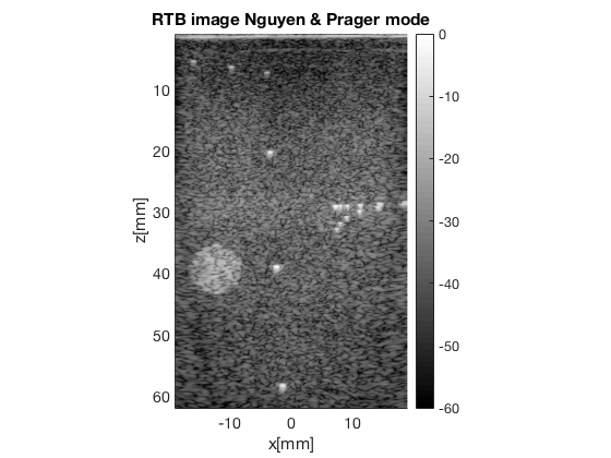
Their model sucessfully removes the artifact at focus (29.6 mm)!

RTB using our introduced model, the hybrid transmit delay model.

This is a simple model using conventional spherical transmit delay, but we assuming PW ware propagation around focus We firs set up the beamforming to create all the images created from each transmit.

mid_RTB_with_plane_model=midprocess.das();
mid_RTB_with_plane_model.dimension = dimension.receive();
mid_RTB_with_plane_model.transmit_delay_model = transmit_delay_model.hybrid;

%Optionally set the margin of the region around focus to use PW tx delay
mid_RTB_with_plane_model.pw_margin = 1/1000;

mid_RTB_with_plane_model.channel_data=channel_data;
mid_RTB_with_plane_model.scan=scan_RTB;

mid_RTB_with_plane_model.transmit_apodization.window=uff.window.none;
mid_RTB_with_plane_model.transmit_apodization.f_number = 2;
mid_RTB_with_plane_model.transmit_apodization.MLA = MLA;
mid_RTB_with_plane_model.transmit_apodization.MLA_overlap = 1;
mid_RTB_with_plane_model.transmit_apodization.minimum_aperture = [3.000e-03 3.000e-03];

mid_RTB_with_plane_model.receive_apodization.window=uff.window.boxcar;
mid_RTB_with_plane_model.receive_apodization.f_number=1.7;
b_data_RTB_with_plane=mid_RTB_with_plane_model.go();

USTB General beamformer MEX v1.1.2 .............done!

Show and save the individual transmit image from the unfied model

This creates the image in Fig. 7c.

f556 = figure(556);clf;
img = reshape(b_data_RTB_with_plane.data,scan_RTB.N_z_axis,scan_RTB.N_x_axis,channel_data.N_waves);
imagesc(scan_RTB.x_axis*1000,z_axis*1000,db(abs(img(:,:,tx)./max(max(img(:,:,tx))))));
colormap gray; caxis([-60 0]); axis image;
xlabel('x[mm]');ylabel('z[mm]');
set(gca,'Fontsize',15)
saveas(f556,[ustb_path,'/publications/IUS2018/Rindal_et_al_ASimpleArtifactFreeVirtualSourceModel/Figures/full_image_hybrid_single_tx.eps'],'eps2c')

Adjust the beamforming to apply the tukey window on the individual transmit images

This creates the images in Fig. 8c.

mid_RTB_with_plane_model.transmit_apodization.window=uff.window.tukey25;
b_data_RTB_with_plane=mid_RTB_with_plane_model.go();

f556 = figure(556);clf;
img = reshape(b_data_RTB_with_plane.data,scan_RTB.N_z_axis,scan_RTB.N_x_axis,channel_data.N_waves);
imagesc(scan_RTB.x_axis*1000,z_axis*1000,db(abs(img(:,:,tx)./max(max(img(:,:,tx))))));
colormap gray; caxis([-60 0]); axis image;
xlabel('x[mm]');ylabel('z[mm]');
set(gca,'Fontsize',15)
axis([-2 -0.1 26 33])
saveas(f556,[ustb_path,'/publications/IUS2018/Rindal_et_al_ASimpleArtifactFreeVirtualSourceModel/Figures/hybrid_zoomed_single_tx.eps'],'eps2c')

uff.apodization: Inputs and outputs are unchanged. Skipping process.
USTB General beamformer MEX v1.1.2 .............done!

Adjust the beamforming to create the full RTB image from our hybrid model

mid_RTB_with_plane_model.dimension = dimension.both();
mid_RTB_with_plane_model.transmit_apodization.window=uff.window.tukey25;
b_data_RTB_with_plane=mid_RTB_with_plane_model.go();

% Calculate the transmit apodzation used to compensate image
tx_apod = mid_RTB_with_plane_model.transmit_apodization.data;

% Also compensating with TX transmit apodization as weighting we get the
% final image shown in Fig. 3d and 4d.
b_data_RTB_plane_fix_weighted = uff.beamformed_data(b_data_RTB_with_plane);
b_data_RTB_plane_fix_weighted.data = b_data_RTB_plane_fix_weighted.data...
                                                        .*(1./sum(tx_apod,2));
b_data_RTB_plane_fix_weighted.plot(10,'RTB image with PW hybrid virtual source model');

f459 = figure(459);clf;
imagesc(scan_RTB.x_axis*1000,z_axis*1000,b_data_RTB_plane_fix_weighted.get_image);
colormap gray; caxis([-60 0]); axis image;
xlabel('x[mm]');ylabel('z[mm]');
set(gca,'Fontsize',15)
saveas(f459,[ustb_path,'/publications/IUS2018/Rindal_et_al_ASimpleArtifactFreeVirtualSourceModel/Figures/full_image_hybrid.eps'],'eps2c')
axis([5 12 26 36])
saveas(f459,[ustb_path,'/publications/IUS2018/Rindal_et_al_ASimpleArtifactFreeVirtualSourceModel/Figures/full_image_hybrid_zoomed.eps'],'eps2c')

uff.apodization: Inputs and outputs are unchanged. Skipping process.
uff.apodization: Inputs and outputs are unchanged. Skipping process.
USTB General beamformer MEX v1.1.2 .............done!
uff.apodization: Inputs and outputs are unchanged. Skipping process.

Our simple model also removes the artifact

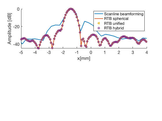
Create Fig. 5. comparing resolution of the scatterer at z = 58.5

f456 = figure(456);clf;
subplot(211);
img_conventional = b_data.get_image;
img_vs = b_data_RTB_weighted.get_image;
img_unified = b_data_RTB_unified_fix_weighted.get_image;
img_hybrid = b_data_RTB_plane_fix_weighted.get_image;
hold all;
plot(scan.x_axis*1000,img_conventional(962,:)-max(img_conventional(962,:)),'LineWidth',2,'DisplayName','Scanline beamforming');
plot(scan_RTB.x_axis*1000,img_vs(962,:)-max(img_vs(962,:)),'LineWidth',2,'DisplayName','RTB spherical');
scatter(scan_RTB.x_axis(:)*1000,img_unified(962,:)-max(img_unified(962,:)),'LineWidth',2,'DisplayName','RTB unified','Marker','<');
scatter(scan_RTB.x_axis*1000,img_hybrid(962,:)-max(img_hybrid(962,:)),'LineWidth',2,'DisplayName','RTB hybrid','Marker','o');
xlim([-5 4]);legend show;
ylabel('Amplitude [dB]');xlabel('x[mm]')

set(gca,'Fontsize',15)
saveas(f456,[ustb_path,'/publications/IUS2018/Rindal_et_al_ASimpleArtifactFreeVirtualSourceModel/Figures/resolution.eps'],'eps2c')

Create plot that was used in the abstract showing the images and the TX delays

The images can be zoomed in on the artifact as we did in the abstract, and we can see that both the Nguyen & Prager model, and our simple PW model sucessfully removes the artifact at focus.

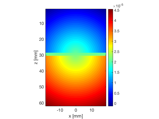
% We are plotting the TX delay used for the center transmit beam
tx_delay_spherical_model = reshape(mid_RTB_spherical_model.transmit_delay,scan_RTB.N_z_axis,...
                                    scan_RTB.N_x_axis,channel_data.N_waves);
tx_delay_unified_model = reshape(mid_RTB_unified_model.transmit_delay,scan_RTB.N_z_axis,...
                                    scan_RTB.N_x_axis,channel_data.N_waves);
tx_delay_hybrid_model = reshape(mid_RTB_with_plane_model.transmit_delay,scan_RTB.N_z_axis,...
                                    scan_RTB.N_x_axis,channel_data.N_waves);

h = figure(100);clf;
b_data_RTB_weighted.plot(subplot(2,3,1),'1a : Virtual source model');
ax(1) = gca;
b_data_RTB_unified_fix_weighted.plot(subplot(2,3,2),'1b : Model from [1]');
ax(2) = gca;
b_data_RTB_plane_fix_weighted.plot(subplot(2,3,3),'1c : Virt. source+PW model');
ax(3) = gca;
linkaxes(ax);
axis([5 12 26 36])

subplot(2,3,4); imagesc(scan_RTB.x_axis*1000, scan_RTB.z_axis*1000, ...
                    tx_delay_spherical_model(:,:,channel_data.N_waves/2));
title('1d: Tx delay virtual source model');xlabel('x [mm]');ylabel('z [mm]');
colorbar; set(gca,'fontsize',14);
subplot(2,3,5); imagesc(scan_RTB.x_axis*1000, scan_RTB.z_axis*1000, ...
                            tx_delay_unified_model(:,:,channel_data.N_waves/2));
title('1e: Tx delay model from [1]');xlabel('x [mm]');ylabel('z [mm]');
colorbar; set(gca,'fontsize',14);
subplot(2,3,6); imagesc(scan_RTB.x_axis*1000, scan_RTB.z_axis*1000, ....
                            tx_delay_hybrid_model(:,:,channel_data.N_waves/2));
title('1f: Tx delay virt. source+PW model');xlabel('x [mm]');ylabel('z [mm]');
colorbar; set(gca,'fontsize',14);%colormap jet;

set(h,'Position',[271    38   843   621]);

% A few trics to get the colormap in the submitted abstract:
% 1. Run the three bottom subplots with colormap jet
% 2. Rerun the three first subplots to get colormap gray

Plot the calculated delays for the 64/128 transmitted wave in Fig. 6.

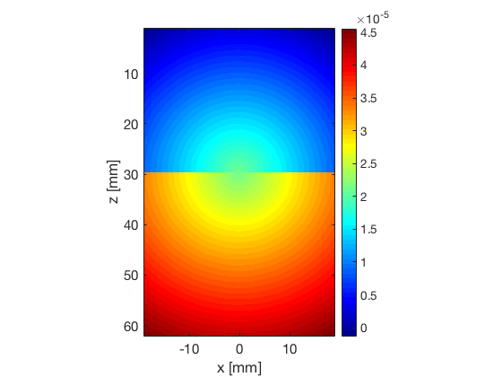
First plot the delay calculated for the spherical model

f66 = figure(66);
imagesc(scan_RTB.x_axis*1000, scan_RTB.z_axis*1000, ...
                    tx_delay_spherical_model(:,:,channel_data.N_waves/2));
colorbar; set(gca,'fontsize',14); xlabel('x [mm]');ylabel('z [mm]');
set(gca,'Fontsize',15)
axis image;
c = caxis;
caxis(c); colormap jet
saveas(f66,[ustb_path,'/publications/IUS2018/Rindal_et_al_ASimpleArtifactFreeVirtualSourceModel/Figures/delay_vs.eps'],'eps2c')

Plot the delay calculated for the unified model

f67 = figure(67);
imagesc(scan_RTB.x_axis*1000, scan_RTB.z_axis*1000, ...
                            tx_delay_unified_model(:,:,channel_data.N_waves/2));
colorbar; set(gca,'fontsize',14); xlabel('x [mm]');ylabel('z [mm]');
set(gca,'Fontsize',15)
axis image;
caxis(c); colormap jet
saveas(f67,[ustb_path,'/publications/IUS2018/Rindal_et_al_ASimpleArtifactFreeVirtualSourceModel/Figures/delay_unified.eps'],'eps2c')

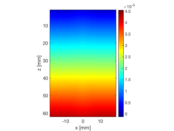
Plot the delay calculated for the hybrid model

f68 = figure(68);
imagesc(scan_RTB.x_axis*1000, scan_RTB.z_axis*1000, ....
                            tx_delay_hybrid_model(:,:,channel_data.N_waves/2));
colorbar; set(gca,'fontsize',14); xlabel('x [mm]');ylabel('z [mm]');
set(gca,'Fontsize',15)
axis image;
caxis(c); colormap jet
saveas(f68,[ustb_path,'/publications/IUS2018/Rindal_et_al_ASimpleArtifactFreeVirtualSourceModel/Figures/delay_hybrid.eps'],'eps2c')

Published with MATLAB® R2018a