Acoustic Radiation Force Imaging from UFF file recorded with the Verasonics ARFI_L7 example
In this example we demonstrate the speckle tracking of displacement created by a shear wave induced with an acoustic "push" pulse. Also known as acoustic radiation force imaging, or share wave elastography. You will need an internet connection to download the data. Otherwise, you can run the ARFI_L7.m Verasonics example and create your own .uff file.
Ole Marius Hoel Rindal olemarius@olemarius.net 15.08.2017
Contents
Reading the channel data from the UFF file
clear all; close all;

% data location
url='http://ustb.no/datasets/';      % if not found data will be downloaded from here
local_path = [ustb_path(),'/data/']; % location of example data on this computer
filename='ARFI_dataset.uff';

% check if the file is available in the local path & downloads otherwise
tools.download(filename, url, local_path);
Reading channel data from the UFF file and print out information about the dataset.
channel_data = uff.read_object([local_path filename],'/channel_data');
channel_data.print_authorship
UFF: reading channel_data [uff.channel_data]
Name: 		 CPWC dataset from a CIRS Elasticity QA Spherical
		 Phantom. The dataset consists of 4 Verasonics
		 _superframes_ with 50 super high framerate plane
		 wave images after an acoustical radiation force
		 push creating share waves. The image has a harder
		 sphere at about x = 10 mm and z = 15 mm
Reference: 	 www.ultrasoundtoolbox.com
Author(s): 	 Ole Marius Hoel Rindal <olemarius@olemarius.net>
		 Fabrice Prieur <fabrice@ifi.uio.no>
Version: 	 1.0.0
Beamform images
First, we need to beamform the images from the channel data. We'll do the usual drill of defining the scan and the beamformer object.
% SCAN
sca=uff.linear_scan();
sca.x_axis = linspace(channel_data.probe.x(1),channel_data.probe.x(end),256).';
sca.z_axis = linspace(0,30e-3,256).';

% BEAMFORMER
bmf=beamformer();
bmf.channel_data=channel_data;
bmf.scan=sca;

bmf.receive_apodization.window=uff.window.tukey50;
bmf.receive_apodization.f_number=1.7;
bmf.receive_apodization.origo=uff.point('xyz',[0, 0, -Inf]);

bmf.transmit_apodization.window=uff.window.tukey50;
bmf.transmit_apodization.f_number=1.7;
bmf.transmit_apodization.origo=uff.point('xyz',[0, 0, -Inf]);

% Do beamforming
b_data=bmf.go({process.das_mex process.coherent_compounding});
Show beamformed images
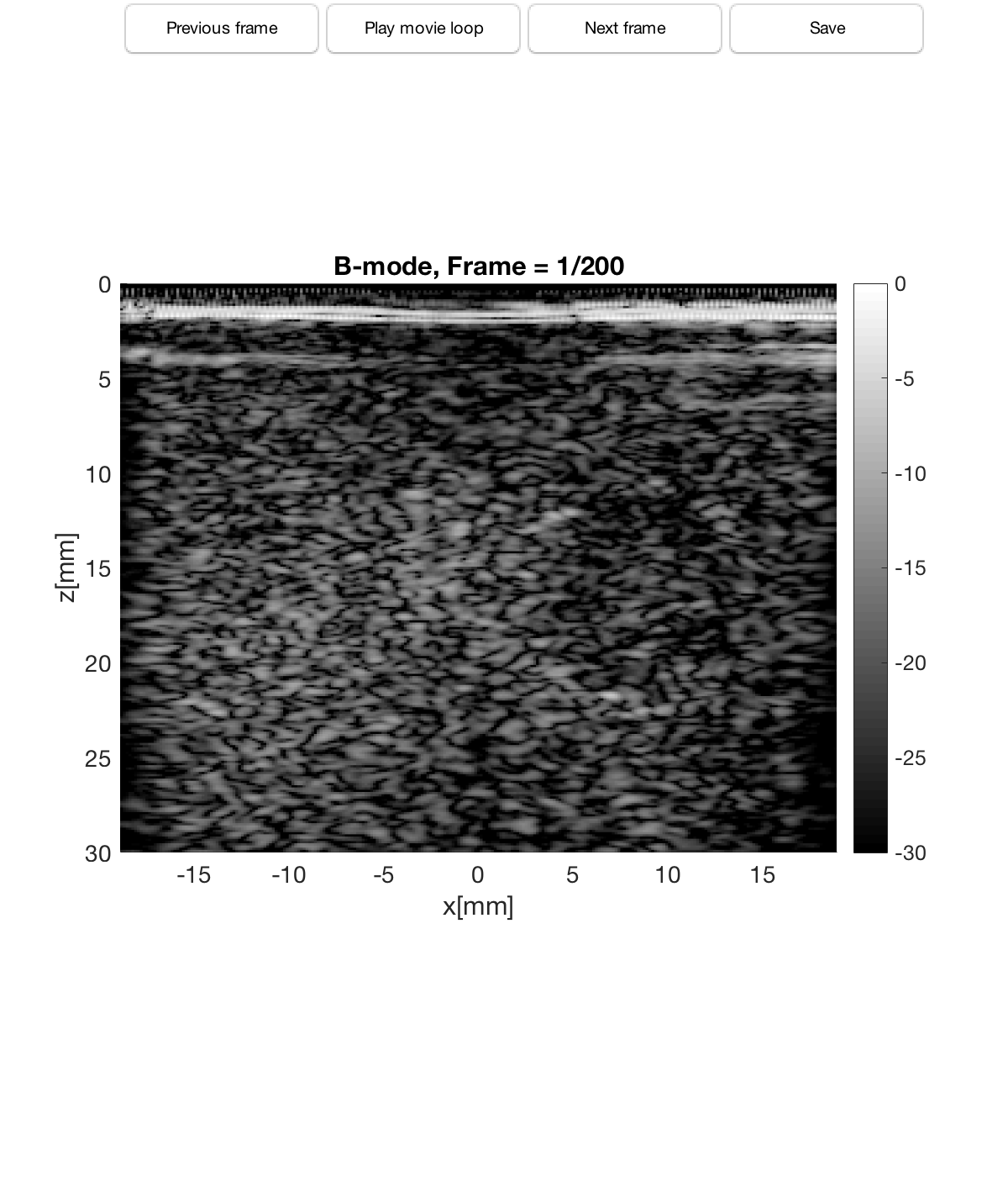
The b-mode images is really not that interesting. The displacement created by the shear waves are to small to be seen. Notice that we barely see a circular structure at about x = 10 and z = 15 mm. This is a sphere in the phantom which is somewhat harder than the surrounding structure.
b_data.plot(1,['B-mode'],[30]);
Estimate displacement
To actually see the shear wave propagation we need to estimate the displacement. This is done using a USTB process called autocorrelation_displacement_estimation. Have a look at its references to see the details.
disp = process.autocorrelation_displacement_estimation();
disp.channel_data = channel_data;
disp.beamformed_data = b_data;
disp.z_gate = 4;        % Nbr of samples to average estimate in depth / z
disp.x_gate = 2;        % Nbr of samples to average estimate in lateral / x
disp.packet_size = 6;   % How many frames to use in the estimate
displacement_estimation = disp.go();
disp.print_reference    % This is the references
disp.print_implemented_by    % Credits to the people who implemented it ;)
Reference:	 Barber, W. D., Eberhard, J. W., & Karr, S. G. (198
		 5). A new time domain technique for velocity measu
		 rements using Doppler ultrasound. IEEE Transaction
		  on Biomedical Engineering, 32(3)Kasai, C., Nameka
		 wa, K., Koyano, A., & Omoto, R. (1985). Real-Time
		 Two-Dimensional Blood Flow Imaging Using an Autoco
		 rrelation Technique. IEEE Transactions on Sonics a
		 nd Ultrasonics, 32(3).Angelsen, B.A.J., & Kristoff
		 ersen, K. (1983). Discrete time estimation of the
		 mean Doppler frequency in ultrasonic blood velocit
		 y measurements. IEEE Transaction on Biomedical Eng
		 ineering, (4).
Implemented by:	 Ole Marius Hoel Rindal <olemarius@olemarius.net>,
		 Thomas B?rstad <thomas.borstad@gmail.com>
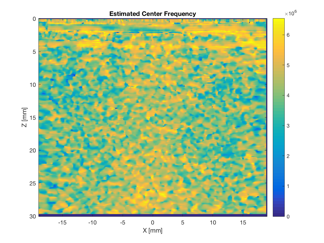
We also have an alternative implementation also estimating the center frequency. This is the modified_autocorrelation_displacement_estimation. Please see the individiual implementations and references for more details.
disp_mod = process.modified_autocorrelation_displacement_estimation();
disp_mod.channel_data = channel_data;
disp_mod.beamformed_data = b_data;
disp_mod.z_gate = 4;        % Nbr of samples to average estimate in depth / z
disp_mod.x_gate = 2;        % Nbr of samples to average estimate in lateral / x
disp_mod.packet_size = 6;   % How many frames to use in the estimate
displacement_estimation_modified = disp_mod.go();
disp_mod.print_reference    % This is the references
disp_mod.print_implemented_by    % Credits to the people who implemented it ;)
Reference:	 Loupas, T., Powers, J. T., & Gill, R. W. (1995). A
		 n Axial Velocity Estimator for Ultrasound Blood Fl
		 ow Imaging, Based on a Full Evaluation of the Dopp
		 ler Equation by Means of a Two-Dimensional Autocor
		 relation Approach. IEEE Transactions on Ultrasonic
		 s, Ferroelectrics and Frequency Control, 42(4).Bar
		 ber, W. D., Eberhard, J. W., & Karr, S. G. (1985).
		  A new time domain technique for velocity measurem
		 ents using Doppler ultrasound. IEEE Transaction on
		  Biomedical Engineering, 32(3)Kasai, C., Namekawa,
		  K., Koyano, A., & Omoto, R. (1985). Real-Time Two
		 -Dimensional Blood Flow Imaging Using an Autocorre
		 lation Technique. IEEE Transactions on Sonics and
		 Ultrasonics, 32(3).Angelsen, B.A.J., & Kristoffers
		 en, K. (1983). Discrete time estimation of the mea
		 n Doppler frequency in ultrasonic blood velocity m
		 easurements. IEEE Transaction on Biomedical Engine
		 ering, (4).
Implemented by:	 Ole Marius Hoel Rindal <olemarius@olemarius.net>,
		 Thomas B?rstad <thomas.borstad@gmail.com>
Display the displacement estimate
Now, we can finally show the estimated displacement. This is nice to visualize as a movie.
In the movie we can clearly see the acoustic radiation force push that creates the share waves. The push is centered at x = 0 mm and z = 14 mm. Notice how the shear waves interacts with the harder spherical structure at x = 10 and z = 15 mm. The wavefront is moving faster through the harder tissue and some complex wavefronts are created.
Notice that we give the figure and the title as arguments to the plot function. The empty brackets [] is because we don't want to specify any dynamic range (well do that with the caxis function). And the 'none' is because we don't want to do any compression of the displacement data
f2 = figure(2);clf;
handle = displacement_estimation.plot(f2,['Displacement'],[],'none');
caxis([-0.1*10^-6 0.2*10^-6]); % Updating the colorbar
colormap(gca(f2),'hot');       % Changing the colormap

f3 = figure(3);clf;
handle = displacement_estimation_modified.plot(f3,['Displacement modified estimation'],[],'none');
caxis([-0.1*10^-6 0.2*10^-6]); % Updating the colorbar
colormap(gca(f3),'hot');       % Changing the colormap
Let's check the estimated center frequency and make sure that it is around 5 MHz as it should be. It is, but is the estimate any better?
figure(4);
imagesc(disp_mod.scan.x_axis*1000,disp_mod.scan.z_axis*1000,disp_mod.estimated_center_frequency(:,:,10));
xlabel('X [mm]');ylabel('Z [mm]');title('Estimated Center Frequency');
colorbar;
We can do it all in once!!
Since the autocorrelation_displacement_estimation is a process, we can trust the default paramters (which are the same as the ones used above) and do the beamforming and the displacement estimation all in one call!
Isn't the USTB great?!
disp = bmf.go({process.das_mex process.coherent_compounding ...
                                process.autocorrelation_displacement_estimation});
Display the displacement Which gives us the same result as above.
f5 = figure(5);clf;
disp.plot(f5,['Displacement'],[],'none');
caxis([-0.1*10^-6 0.2*10^-6]); % Updating the colorbar
colormap(gca(f5),'hot');       % Changing the colormap