Resolution of Delay Multiply And Sum on FI data from an UFF file
by Ole Marius Hoel Rindal olemarius@olemarius.net 28.05.2017
Contents
Setting up file path
To read data from a UFF file the first we need is, you guessed it, a UFF file. We check if it is on the current path and download it from the USTB websever.
clear all; close all;

% data location
url='http://ustb.no/datasets/';      % if not found downloaded from here
local_path = [ustb_path(),'/data/']; % location of example data
addpath(local_path);

% Choose dataset
filename='Alpinion_L3-8_FI_hyperechoic_scatterers.uff';

% check if the file is available in the local path or downloads otherwise
tools.download(filename, url, local_path);
Reading channel data from UFF file
uff_file=uff(filename)
channel_data=uff_file.read('/channel_data');
uff_file =

  uff with properties:

    filename: 'Alpinion_L3-8_FI_hyperechoic_scatterers.uff'
     version: 'v1.0.1'
        mode: 'append'
     verbose: 1

UFF: reading channel_data [uff.channel_data]
UFF: reading sequence [uff.wave]
Processed 256/256
%Print info about the dataset
channel_data.print_info
Name: 		 FI dataset of hyperechoic cyst and points
		 scatterers recorded on an Alpinion scanner with a
		 L3-8 Probe from a CIRS General Purpose Ultrasound
		 Phantom
Reference: 	 www.ultrasoundtoolbox.com
Author(s): 	 Ole Marius Hoel Rindal <olemarius@olemarius.net>
		 Muyinatu Lediju Bell <mledijubell@jhu.edu>
Version: 	 1.0.2
Define Scan
Define the image coordinates we want to beamform in the scan object. Notice that we need to use quite a lot of samples in the z-direction. This is because the DMAS creates an "artificial" second harmonic signal, so we need high enough sampling frequency in the image to get a second harmonic signal.
z_axis=linspace(25e-3,45e-3,1024).';
sca=uff.linear_scan();
idx = 1;
for n=1:numel(channel_data.sequence)
    sca(n)=uff.linear_scan(channel_data.sequence(n).source.x,z_axis);
end
Set up delay part of beamforming
setting up and running the delay part of the beamforming
bmf=beamformer();
bmf.channel_data=channel_data;
bmf.scan=sca;

bmf.receive_apodization.window=uff.window.boxcar;
bmf.receive_apodization.f_number=1.7;
bmf.receive_apodization.apex.distance=Inf;

bmf.transmit_apodization.window=uff.window.none;
b_data=bmf.go({process.delay_matlab_light process.stack});
Create the DMAS image using the delay_multiply_and_sum process
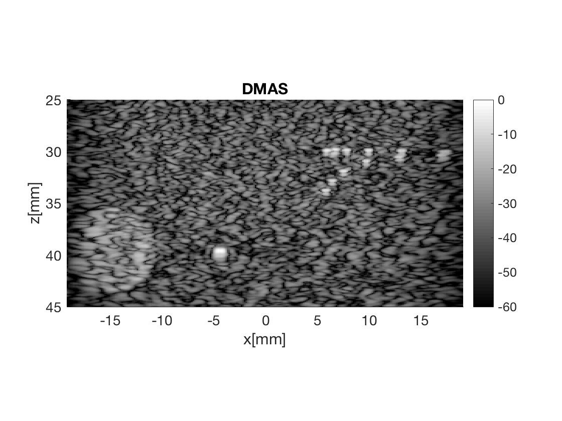
dmas = process.delay_multiply_and_sum();
dmas.dimension = dimension.receive();
dmas.receive_apodization = bmf.receive_apodization;
dmas.transmit_apodization = bmf.transmit_apodization;
dmas.beamformed_data = b_data;
dmas.channel_data = channel_data;
dmas.scan = sca
b_data_dmas = dmas.go();        % Launch beamformer
b_data_dmas.plot(100,'DMAS');   % Display image
dmas =

  delay_multiply_and_sum with properties:

               dimension: receive
            channel_data: [1×1 uff.channel_data]
     receive_apodization: [1×1 uff.apodization]
    transmit_apodization: [1×1 uff.apodization]
                    scan: [1×256 uff.linear_scan]
         beamformed_data: [1×1 uff.beamformed_data]
                    name: 'Delay Multiply and Sum'
               reference: 'Matrone, G., Savoia, A. S., & Magenes, G. (2015...'
          implemented_by: {'Ole Marius Hoel Rindal <olemarius@olemarius.net>'}
                 version: 'v1.0.2'

Warning: If the result looks funky, you might need to tune the filter paramters
of DMAS. Use the plot to check that everything is OK.
Beamform DAS image
Notice that we just need to sum the data since it is allready delayed
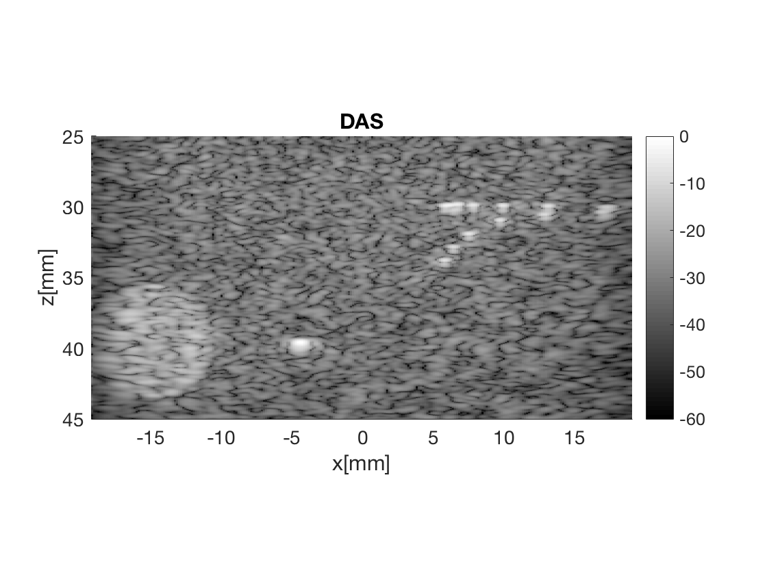
das = process.coherent_compounding();
das.beamformed_data = b_data;

b_data_das=das.go();
b_data_das.plot(2,'DAS');
Plot both images in same plot
Plot both in same plot with connected axes, try to zoom!
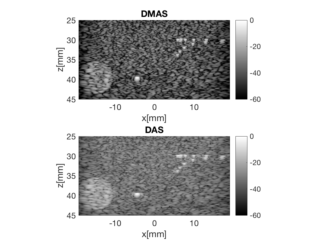
f3 = figure(3);clf
b_data_dmas.plot(subplot(2,1,1),'DMAS'); % Display image
ax(1) = gca;
b_data_das.plot(subplot(2,1,2),'DAS'); % Display image
ax(2) = gca;
linkaxes(ax);
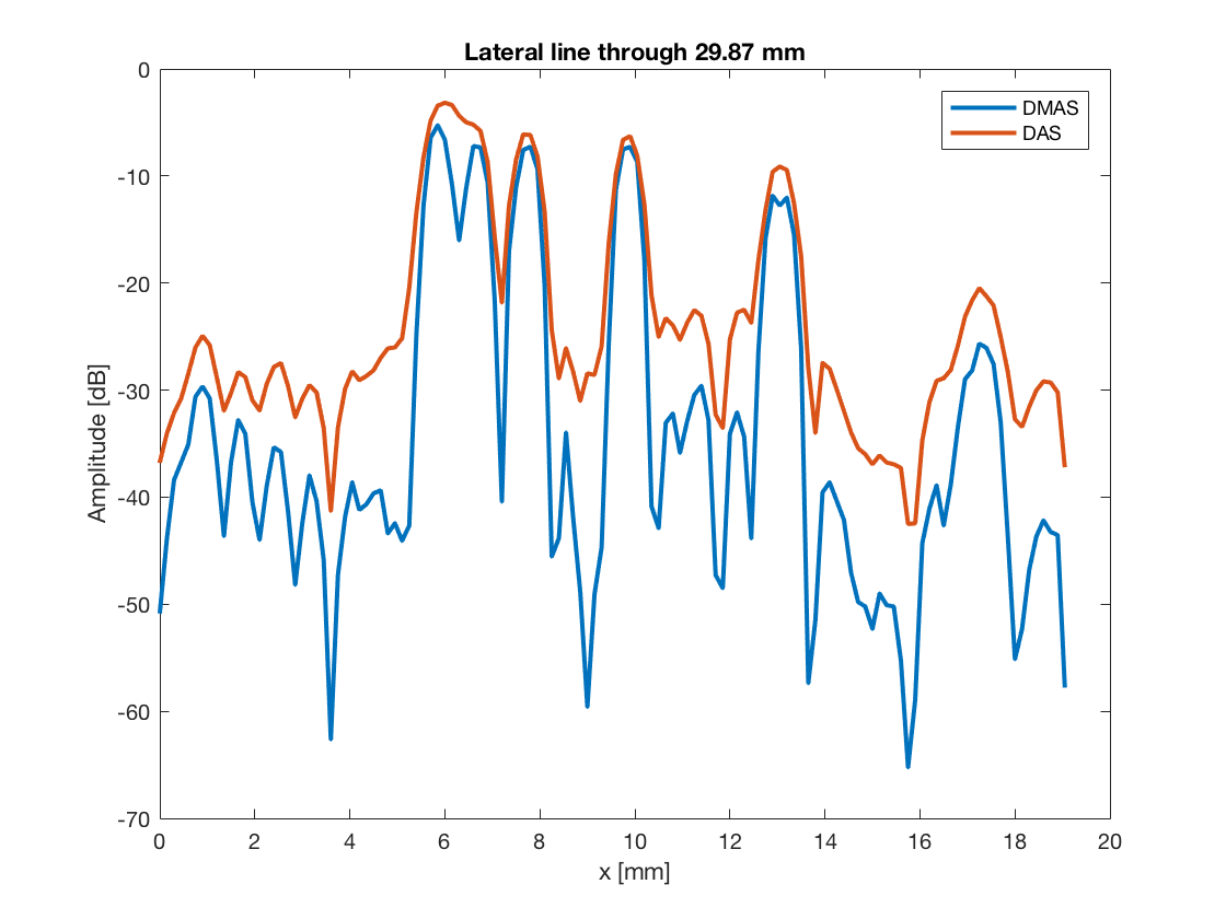
Compare resolution
Plot the lateral line through some of the scatterers
% Let's get the images as a N_z_axis x N_x_axis image
dmas_img = b_data_dmas.get_image();
das_img = b_data_das.get_image();
So that we can plot the line through the group of scatterers
line_idx = 250;
figure(4);clf;
plot(b_data_dmas.scan.x_axis*10^3,dmas_img(line_idx,:),...
                               'DisplayName','DMAS','LineWidth',2);hold on;
plot(b_data_das.scan.x_axis*10^3,das_img(line_idx,:),...
                               'DisplayName','DAS','LineWidth',2);
xlabel('x [mm]');xlim([0 20]);ylabel('Amplitude [dB]');legend show
title(sprintf('Lateral line through %.2f mm',...
                                  b_data_dmas.scan.z_axis(line_idx)*10^3));
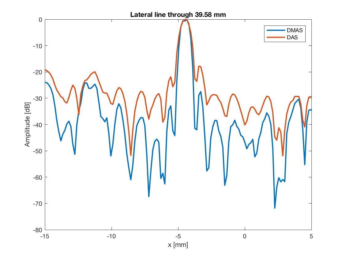
%So that we can plot the line through the aingle scatterer
line_idx = 747;
figure(5);clf;
plot(b_data_dmas.scan.x_axis*10^3,dmas_img(line_idx,:),...
                                'DisplayName','DMAS','LineWidth',2);hold on;
plot(b_data_das.scan.x_axis*10^3,das_img(line_idx,:),...
                                'DisplayName','DAS','LineWidth',2);
xlabel('x [mm]');xlim([-15 5]);ylabel('Amplitude [dB]');legend show
title(sprintf('Lateral line through %.2f mm',...
                                  b_data_dmas.scan.z_axis(line_idx)*10^3));