Contents
- Create the figures from the experimental dynamic range phantom
- Load the data
- Print authorship and citation details for the dataset
- Display and save the images from all beamformers under study
- DAS
- CF
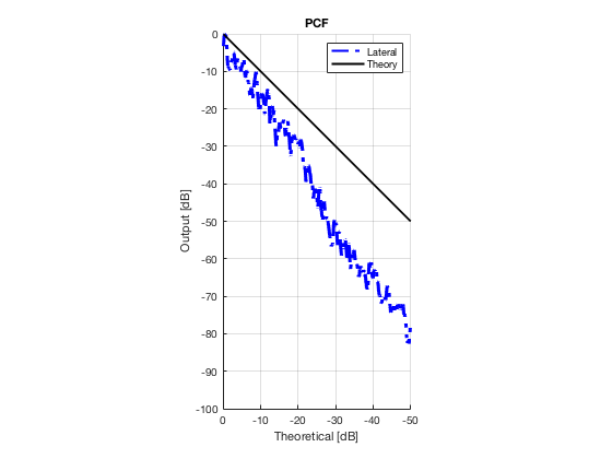
- PCF
- GCF
- MV
- F-DMAS
- EBMV
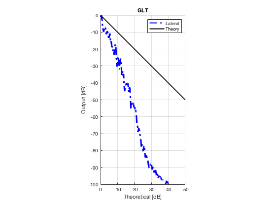
- GLT
- Put the images in a cell array.
- Add the path to the functions used in the evaluation
- Plot lateral graident in db vs. db plot.
- Measure contrast
- Run the Dynamic Range Test (DRT)
- Plotting correlation plot between CR improvement and DRT with all 8 beamforming (including GLT)
- Plotting correlation plot between CR improvement and DRT with all 7 methods (excluding GLT)
- Save the data to a file to read parts of the results to be plotted with the simulated data
Create the figures from the experimental dynamic range phantom
For the publication Rindal, O. M. H., Austeng, A., Fatemi, A., & Rodriguez-Molares, A. (2018). The effect of dynamic range alterations in the estimation of contrast. Submitted to IEEE Transactions on Ultrasonics, Ferroelectrics, and Frequency Control.
Author: Ole Marius Hoel Rindal olemarius@olemarius.net 05.06.18 updated for revised version of manuscript 12.03.19
clear all;
close all;
addpath([ustb_path,filesep,'publications',filesep,'DynamicRange',filesep,'functions',filesep])
Warning: The file
'/Applications/MATLAB_R2018a.app/toolbox/matlab/codetools/private/evalmxdom.m'
could not be cleared because it contains MATLAB code that is currently
executing.
Warning: The file
'/Applications/MATLAB_R2018a.app/toolbox/matlab/codetools/mdbpublish.m' could
not be cleared because it contains MATLAB code that is currently executing.
Warning: The file
'/Applications/MATLAB_R2018a.app/toolbox/matlab/codetools/publish.p' could not
be cleared because it contains MATLAB code that is currently executing.
Warning: The file
'/Users/omrindal/Development/USTB_dynamic_range_revision_final/publications/DynamicRange/create_figures_from_experimental.m'
could not be cleared because it contains MATLAB code that is currently
executing.
Warning: The file
'/Applications/MATLAB_R2018a.app/toolbox/matlab/codetools/private/evalmxdom.m'
could not be cleared because it contains MATLAB code that is currently
executing.
Warning: The file
'/Applications/MATLAB_R2018a.app/toolbox/matlab/codetools/mdbpublish.m' could
not be cleared because it contains MATLAB code that is currently executing.
Warning: The file
'/Applications/MATLAB_R2018a.app/toolbox/matlab/codetools/publish.p' could not
be cleared because it contains MATLAB code that is currently executing.
Warning: The file
'/Users/omrindal/Development/USTB_dynamic_range_revision_final/publications/DynamicRange/create_figures_from_experimental.m'
could not be cleared because it contains MATLAB code that is currently
executing.
Load the data
filename = 'experimental_STAI_dynamic_range.uff';
url='http://ustb.no/datasets/';      % if not found downloaded from here

% checks if the data is in your data path, and downloads it otherwise.
% The defaults data path is under USTB's folder, but you can change this
% by setting an environment variable with setenv(DATA_PATH,'the_path_you_want_to_use');
tools.download(filename, url, data_path);

channel_data = uff.channel_data();
channel_data.read([data_path,filesep,filename],'/channel_data')

b_data_das = uff.beamformed_data();
b_data_cf = uff.beamformed_data();
b_data_pcf = uff.beamformed_data();
b_data_gcf = uff.beamformed_data();
b_data_mv = uff.beamformed_data();
b_data_ebmv = uff.beamformed_data();
b_data_dmas = uff.beamformed_data();

b_data_das.read([data_path,filesep,filename],'/b_data_das');
b_data_cf.read([data_path,filesep,filename],'/b_data_cf');
b_data_pcf.read([data_path,filesep,filename],'/b_data_pcf');
b_data_gcf.read([data_path,filesep,filename],'/b_data_gcf');
b_data_mv.read([data_path,filesep,filename],'/b_data_mv');
b_data_ebmv.read([data_path,filesep,filename],'/b_data_ebmv');
b_data_dmas.read([data_path,filesep,filename],'/b_data_dmas');
UFF: reading channel_data [uff.channel_data]
UFF: reading sequence [uff.wave] [====================] 100%
UFF: reading /b_data_das [uff.beamformed_data]
UFF: reading /b_data_cf [uff.beamformed_data]
UFF: reading /b_data_pcf [uff.beamformed_data]
UFF: reading /b_data_gcf [uff.beamformed_data]
UFF: reading /b_data_mv [uff.beamformed_data]
UFF: reading /b_data_ebmv [uff.beamformed_data]
UFF: reading /b_data_dmas [uff.beamformed_data]
Print authorship and citation details for the dataset
channel_data.print_authorship
Name: 		 v2 Experimental dynamic range phantom. Recorded
		 on a Verasonics Vantage 256 with a L11 probe. See
		 the reference for details
Reference: 	 Rindal, O. M. H., Austeng, A., Fatemi, A., &
		 Rodriguez-Molares, A. (2018). The effect of
		 dynamic range transformations in the estimation
		 of contrast. Submitted to IEEE Transactions on
		 Ultrasonics, Ferroelectrics, and Frequency
		 Control.
Author(s): 	 Alfonso Rodriguez-Molares <alfonso.r.molares@ntnu.no>
		 Ali Fatemi <ali.fatemi@ntnu.no>
		 Ole Marius Hoel Rindal <omrindal@ifi.uio.no
Version: 	 1.0.1
Display and save the images from all beamformers under study
mkdir([ustb_path,filesep,'publications/DynamicRange/figures/experimental/'])
Warning: Directory already exists.
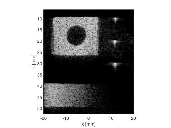
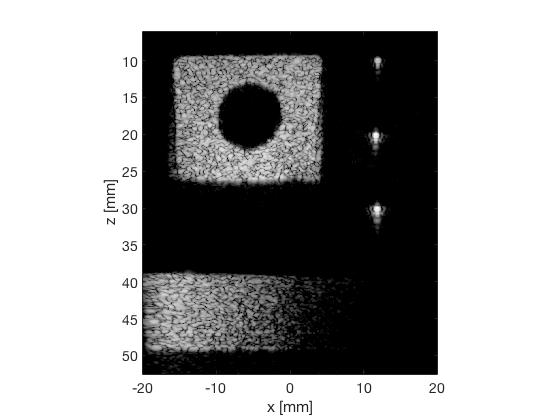
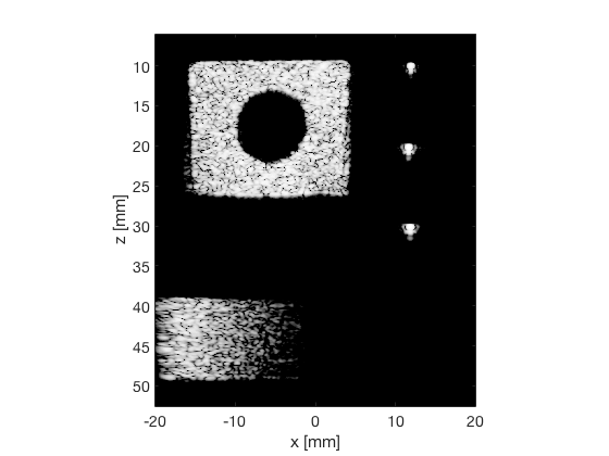
DAS
das_img = b_data_das.get_image('none');
das_img = db(abs(das_img./max(das_img(:)))); % Normalize on max
f1 = figure(1);clf;
imagesc(b_data_das.scan.x_axis*1000,b_data_das.scan.z_axis*1000,das_img);
colormap gray;caxis([-60 0]);axis image;xlabel('x [mm]');ylabel('z [mm]');
set(gca,'FontSize',14);
saveas(f1,[ustb_path,filesep,'publications/DynamicRange/figures/experimental/DAS'],'eps2c')
saveas(f1,[ustb_path,filesep,'publications/DynamicRange/figures/experimental/DAS'],'png')
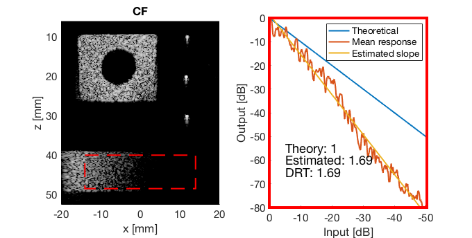
CF
cf_img = b_data_cf.get_image('none');
cf_img = db(abs(cf_img./max(cf_img(:)))); % Normalize on max
f2 = figure(2);
imagesc(b_data_das.scan.x_axis*1000,b_data_das.scan.z_axis*1000,cf_img);
colormap gray;caxis([-60 0]);axis image;xlabel('x [mm]');ylabel('z [mm]');
set(gca,'FontSize',14);
saveas(f2,[ustb_path,filesep,'publications/DynamicRange/figures/experimental/CF'],'eps2c')
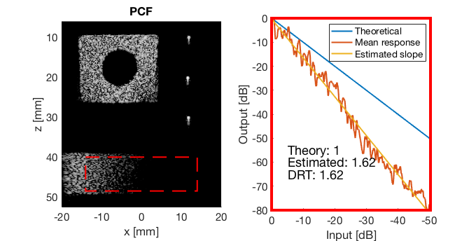
PCF
pcf_img = b_data_pcf.get_image('none');
pcf_img = db(abs(pcf_img./max(pcf_img(:)))); % Normalize on max
f3 = figure(3);clf;
imagesc(b_data_das.scan.x_axis*1000,b_data_das.scan.z_axis*1000,pcf_img);
colormap gray;caxis([-60 0]);axis image;xlabel('x [mm]');ylabel('z [mm]');
set(gca,'FontSize',14);
saveas(f3,[ustb_path,filesep,'publications/DynamicRange/figures/experimental/PCF'],'eps2c')
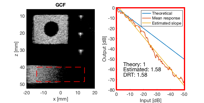
GCF
gcf_img = b_data_gcf.get_image('none');
gcf_img = db(abs(gcf_img./max(gcf_img(:)))); % Normalize on max
f4 = figure(4);
imagesc(b_data_das.scan.x_axis*1000,b_data_das.scan.z_axis*1000,gcf_img);
colormap gray;caxis([-60 0]);axis image;xlabel('x [mm]');ylabel('z [mm]');
set(gca,'FontSize',14);
saveas(f4,[ustb_path,filesep,'publications/DynamicRange/figures/experimental/GCF'],'eps2c')

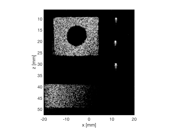
MV
mv_img = b_data_mv.get_image('none');
mv_img = db(abs(mv_img./max(mv_img(:)))); % Normalize on max
f5 = figure(6);clf;
imagesc(b_data_das.scan.x_axis*1000,b_data_das.scan.z_axis*1000,mv_img);
colormap gray;caxis([-60 0]);axis image;xlabel('x [mm]');ylabel('z [mm]');
set(gca,'FontSize',14);
saveas(f5,[ustb_path,filesep,'publications/DynamicRange/figures/experimental/MV'],'eps2c')
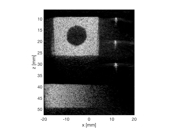
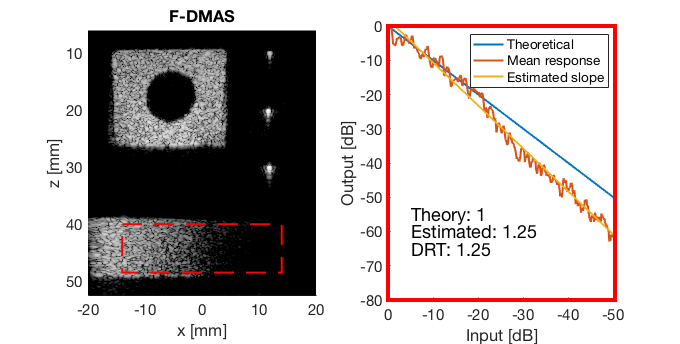
F-DMAS
dmas_img = b_data_dmas.get_image('none');
dmas_img = db(abs(dmas_img./max(dmas_img(:)))); % Normalize on max
f7 = figure(7);clf;
imagesc(b_data_das.scan.x_axis*1000,b_data_das.scan.z_axis*1000,dmas_img);
colormap gray;caxis([-60 0]);axis image;xlabel('x [mm]');ylabel('z [mm]');
set(gca,'FontSize',14);
saveas(f7,[ustb_path,filesep,'publications/DynamicRange/figures/experimental/DMAS'],'eps2c')
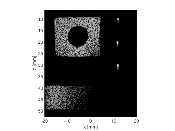
EBMV
ebmv_img = b_data_ebmv.get_image('none');
ebmv_img = db(abs(ebmv_img./max(ebmv_img(:)))); % Normalize on max
f6 = figure(8);clf;
imagesc(b_data_das.scan.x_axis*1000,b_data_das.scan.z_axis*1000,ebmv_img);
colormap gray;caxis([-60 0]);axis image;xlabel('x [mm]');ylabel('z [mm]');
set(gca,'FontSize',14);
saveas(f6,[ustb_path,filesep,'publications/DynamicRange/figures/experimental/EBMV'],'eps2c')
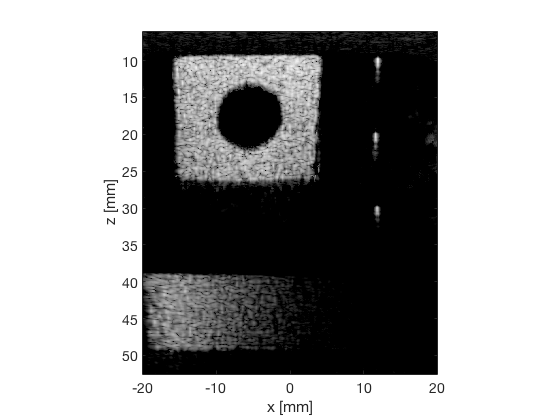
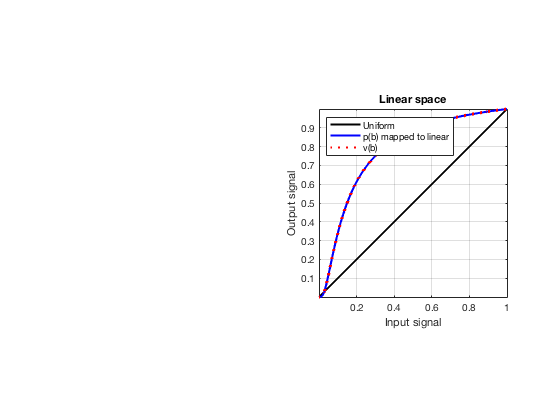
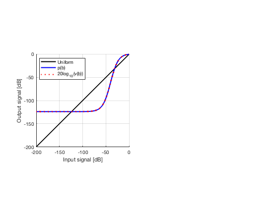
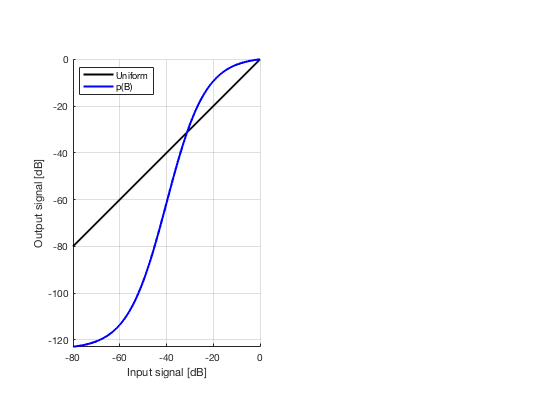
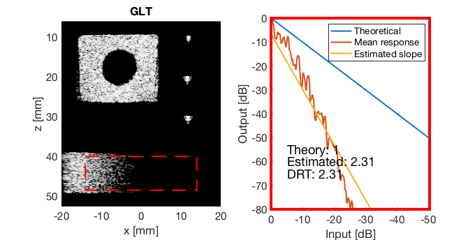
GLT
glt_s = postprocess.scurve_gray_level_transform();
glt_s.a = 0.12;
glt_s.b = -40;
glt_s.c = 0.008;

glt_s.plot_functions = 1;
glt_s.input = b_data_das;
glt_s.scan = b_data_das.scan;
b_data_glt = glt_s.go();

glt_img = b_data_glt.get_image('none');
glt_img = db(abs(glt_img./max(glt_img(:))));
f9 = figure(9);clf;
imagesc(b_data_das.scan.x_axis*1000,b_data_das.scan.z_axis*1000,glt_img);
colormap gray;caxis([-60 0]);axis image;xlabel('x [mm]');ylabel('z [mm]');
set(gca,'FontSize',14);
saveas(f9,[ustb_path,filesep,'publications/DynamicRange/figures/experimental/GLT'],'eps2c')
Put the images in a cell array.
Put both the dB image and the signal before envelope detection
image.all{1} = das_img;
image.all_signal{1} = double(b_data_das.get_image('none'));
image.all_signal{1} = (image.all_signal{1}./max(image.all_signal{1}(:)));
image.tags{1} = 'DAS';
image.all{2} = mv_img;
image.all_signal{2} = double(b_data_mv.get_image('none'));
image.all_signal{2} = (image.all_signal{2}./max(image.all_signal{2}(:)));
image.tags{2} = 'MV';
image.all{3} = ebmv_img;
image.all_signal{3} = double(b_data_ebmv.get_image('none'));
image.all_signal{3} = (image.all_signal{3}./max(image.all_signal{3}(:)));
image.tags{3} = 'EBMV';
image.all{4} = dmas_img;
image.all_signal{4} = double(b_data_dmas.get_image('none'));
image.all_signal{4} = (image.all_signal{4}./max(image.all_signal{4}(:)));
image.tags{4} = 'F-DMAS';
image.all{5} = cf_img;
image.all_signal{5} = double(b_data_cf.get_image('none'));
image.all_signal{5} = (image.all_signal{5}./max(image.all_signal{5}(:)));
image.tags{5} = 'CF';
image.all{6} = gcf_img;
image.all_signal{6} = double(b_data_gcf.get_image('none'));
image.all_signal{6} = (image.all_signal{6}./max(image.all_signal{6}(:)));
image.tags{6} = 'GCF';
image.all{7} = pcf_img;
image.all_signal{7} = double(b_data_pcf.get_image('none'));
image.all_signal{7} = (image.all_signal{7}./max(image.all_signal{7}(:)));
image.tags{7} = 'PCF';
image.all{8} = glt_img;
image.all_signal{8} = double(b_data_glt.get_image('none'));
image.all_signal{8} = (image.all_signal{8}./max(image.all_signal{8}(:)));
image.tags{8} = 'GLT';
Add the path to the functions used in the evaluation
addpath functions

% Add the colors to be used using "linspecer" colors
colors=    [0.9047    0.1918    0.1988; ...
            0.2941    0.5447    0.7494; ...
            0.3718    0.7176    0.3612; ...
            1.0000    0.5482    0.1000; ...
            0.8650    0.8110    0.4330; ...
            0.6859    0.4035    0.2412; ...
            0.9718    0.5553    0.7741; ...
            0.6400    0.6400    0.6400];
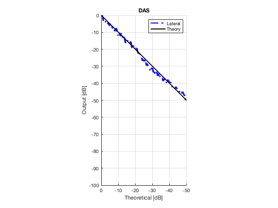
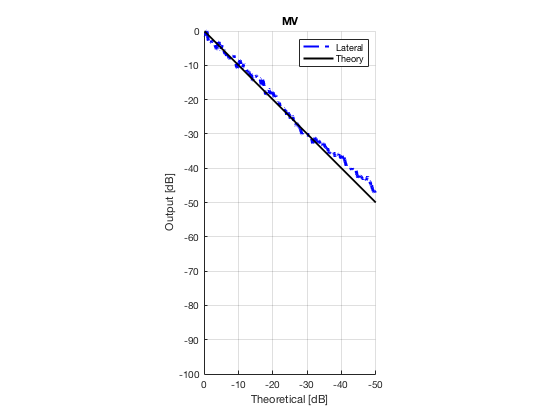
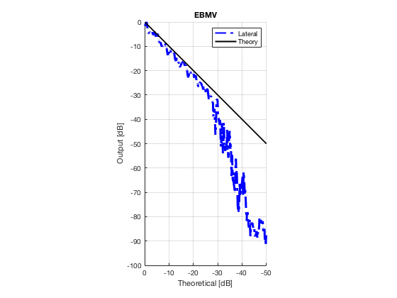
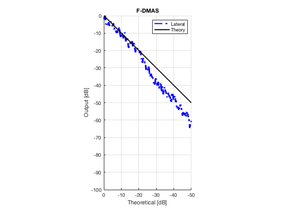
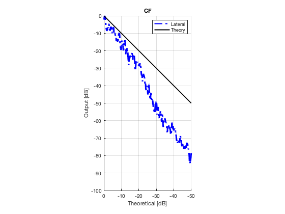
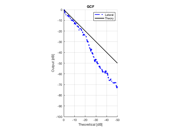
Plot lateral graident in db vs. db plot.
NB! The final figure is plotted together with the simulated data in the create_figures_from_simulation.m script. We are just saving these values for now.
[meanLinesLateral,x_axis] = getMeanLateralLines(b_data_das,image,39,48.5,-14,14);
mask_lateral=abs(b_data_das.scan.x_axis)<14e-3;

theory_lateral = (-1.8*(b_data_das.scan.x_axis(mask_lateral)+14*10^-3))*10^3;

mkdir([ustb_path,filesep,'publications/DynamicRange/figures/experimental/gradient/'])

for i = 1:length(image.all)
    f88 = figure(8888+i);clf;hold all;
    plot(theory_lateral,meanLinesLateral.all{i}-max(meanLinesLateral.all{i}),...
            'LineStyle','-.','Linewidth',2,'Color','b','DisplayName','Lateral');
    plot(theory_lateral,theory_lateral,'LineStyle','-','Linewidth',2,'Color',...
                                                    'k','DisplayName','Theory');
    set(gca, 'XDir','reverse');title(image.tags{i});
    axis image
    legend show
    ylim([-100 0])
    xlim([-50 0])
    grid on
    xlabel('Theoretical [dB]');
    ylabel('Output [dB]');
    saveas(f88,[ustb_path,filesep,...
    'publications/DynamicRange/figures/experimental/gradient/',image.tags{i}],'eps2c')
end
Warning: Directory already exists.
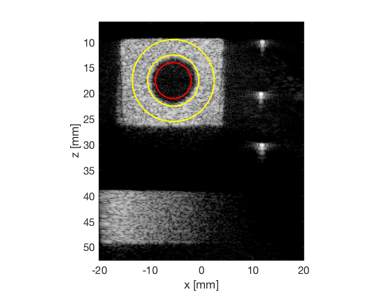
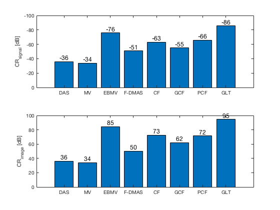
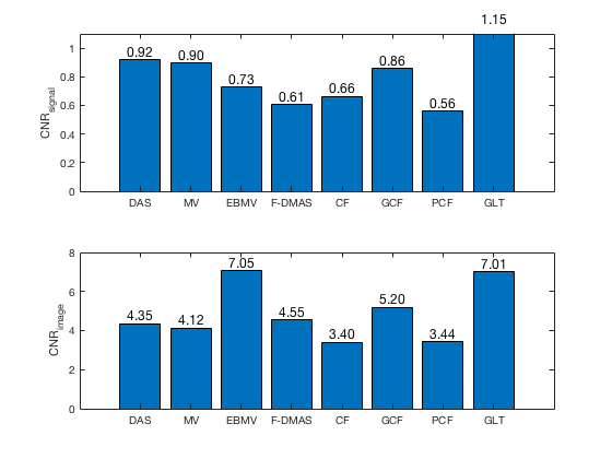
Measure contrast
Once again we are just saving the values to make the final plot combined with the simulated data in the create_figures_from_simulation.m
[CR_signal_exp, CR_signal_dagger, CR_image_exp, CNR_signal_exp, CNR_image_exp] ...
    = measureContrast(b_data_das,image,-5.5,17.5,3.5,5,8,[ustb_path,filesep,...
    'publications/DynamicRange/figures/experimental/DAS_cyst_indicated']);

f9 = figure;
subplot(211);
bar([10*log10(CR_signal_exp)])
set(gca,'XTick',linspace(1,length(image.tags),length(image.tags)))
set(gca,'XTickLabel',image.tags)
ylabel('CR_{signal} [dB]');
x_pos = [1 2 3 4 5 6 7 8];
text(x_pos,double(10*log10(CR_signal_exp(:))),num2str(round(10*log10(CR_signal_exp(:))),'%d'),...
    'HorizontalAlignment','center',...
    'VerticalAlignment','bottom',...
    'FontSize',12)
set(gca,'Ydir','reverse')

subplot(212);
bar([CR_image_exp])
set(gca,'XTick',linspace(1,length(image.tags),length(image.tags)))
set(gca,'XTickLabel',image.tags)
ylabel('CR_{image} [dB]');
x_pos = [1 2 3 4 5 6 7 8];
text(x_pos,double(CR_image_exp(:)),num2str(round(CR_image_exp(:)),'%d'),...
    'HorizontalAlignment','center',...
    'VerticalAlignment','bottom',...
    'FontSize',12)

saveas(f9,[ustb_path,filesep,'publications/DynamicRange/figures/experimental/CR'],'eps2c')

f77 = figure(77);
subplot(211);
bar([CNR_signal_exp])
set(gca,'XTick',linspace(1,length(image.tags),length(image.tags)))
set(gca,'XTickLabel',image.tags)
ylabel('CNR_{signal}');
x_pos = [1 2 3 4 5 6 7 8];
text(x_pos,double(CNR_signal_exp(:)),num2str((CNR_signal_exp(:)),'%.2f'),...
    'HorizontalAlignment','center',...
    'VerticalAlignment','bottom',...
    'FontSize',12)
ylim([0 1.1])

subplot(212);
bar([CNR_image_exp])
set(gca,'XTick',linspace(1,length(image.tags),length(image.tags)))
set(gca,'XTickLabel',image.tags)
ylabel('CNR_{image}');
x_pos = [1 2 3 4 5 6 7 8];
text(x_pos,double(CNR_image_exp(:)),num2str((CNR_image_exp(:)),'%.2f'),...
    'HorizontalAlignment','center',...
    'VerticalAlignment','bottom',...
    'FontSize',12)

saveas(f77,[ustb_path,filesep,'publications/DynamicRange/figures/experimental/CNR'],'eps2c')
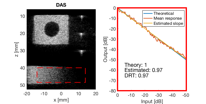
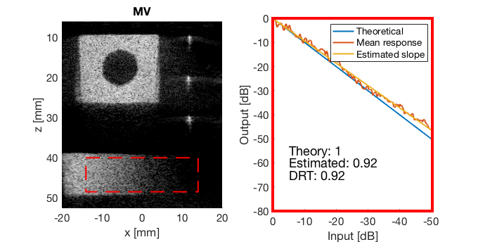
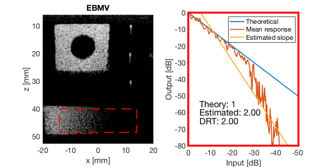
Run the Dynamic Range Test (DRT)
mkdir([ustb_path,filesep,'publications/DynamicRange/figures/experimental/dynamic_range_test/']);
drt{1} = tools.dynamic_range_test(channel_data,b_data_das,'DAS');
set(gcf,'Position',[360 354 680 344])
saveas(gcf,[ustb_path,filesep,'publications/DynamicRange/figures/experimental/dynamic_range_test/','DAS_exp'],'eps2c');
drt{2} = tools.dynamic_range_test(channel_data,b_data_mv,'MV');
set(gcf,'Position',[360 354 680 344])
saveas(gcf,[ustb_path,filesep,'publications/DynamicRange/figures/experimental/dynamic_range_test/','MV'],'eps2c');
drt{3} = tools.dynamic_range_test(channel_data,b_data_ebmv,'EBMV');
set(gcf,'Position',[360 354 680 344])
saveas(gcf,[ustb_path,filesep,'publications/DynamicRange/figures/experimental/dynamic_range_test/','EBMV'],'eps2c');
drt{4} = tools.dynamic_range_test(channel_data,b_data_dmas,'F-DMAS');
set(gcf,'Position',[360 354 680 344])
saveas(gcf,[ustb_path,filesep,'publications/DynamicRange/figures/experimental/dynamic_range_test/','F-DMAS'],'eps2c');
drt{5} = tools.dynamic_range_test(channel_data,b_data_cf,'CF');
set(gcf,'Position',[360 354 680 344])
saveas(gcf,[ustb_path,filesep,'publications/DynamicRange/figures/experimental/dynamic_range_test/','CF'],'eps2c');
drt{6} = tools.dynamic_range_test(channel_data,b_data_gcf,'GCF');
set(gcf,'Position',[360 354 680 344])
saveas(gcf,[ustb_path,filesep,'publications/DynamicRange/figures/experimental/dynamic_range_test/','GCF'],'eps2c');
drt{7} = tools.dynamic_range_test(channel_data,b_data_pcf,'PCF');
set(gcf,'Position',[360 354 680 344])
saveas(gcf,[ustb_path,filesep,'publications/DynamicRange/figures/experimental/dynamic_range_test/','PCF'],'eps2c');
drt{8} = tools.dynamic_range_test(channel_data,b_data_glt,'GLT');
set(gcf,'Position',[360 354 680 344])
saveas(gcf,[ustb_path,filesep,'publications/DynamicRange/figures/experimental/dynamic_range_test/','GLT'],'eps2c')
Warning: Directory already exists.
DRT_value_exp = [drt{1:end}];
cr_improvement = (CR_image_exp - CR_image_exp(1));
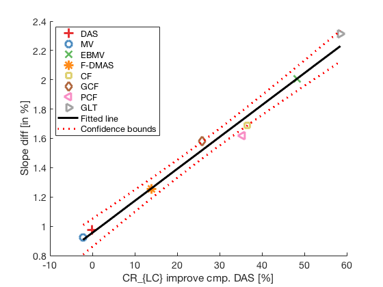
Plotting correlation plot between CR improvement and DRT with all 8 beamforming (including GLT)
lmd_sim_slope = fitlm(cr_improvement(1:8),DRT_value_exp(1:8))

lmd_sim_slope.Rsquared.Ordinary
lmd_sim_slope.Rsquared.Adjusted

f113 = figure(114);clf;hold all;
linespes = '+ox*sd<>';
for i = 1:length(image.all)
    plot(cr_improvement(i),DRT_value_exp(i),linespes(i),'Color',colors(i,:),'MarkerSize',10);
end
lmd_sim_slope.plot
hline = findobj(gcf, 'type', 'line');
set(hline,'LineWidth',3);
set(hline(3),'Color',[0 0 0]);
set(hline(3),'DisplayName','Fitted line');
title('')
xlabel('CR_{LC} improve cmp. DAS [%]');%xlim([-5 75]);
ylabel('Slope diff [in %]');%ylim([-50 5]);
text(80,10,sprintf('R-Squared: %.2f',lmd_sim_slope.Rsquared.Ordinary),'FontSize',18);
text(80,0,sprintf('R-Squared adj: %.2f',lmd_sim_slope.Rsquared.Adjusted),'FontSize',18);
set(gca,'FontSize',14);
delete(hline(4));
legend();
hLegend = findobj(gcf, 'Type', 'Legend');
legend show
legend([{image.tags{1:8}} hLegend.String],'Location','nw');

saveas(f113,[ustb_path,filesep,'publications/DynamicRange/figures/experimental/correlation_experimental'],'eps2c')
lmd_sim_slope =


Linear regression model:
    y ~ 1 + x1

Estimated Coefficients:
                   Estimate       SE        tStat       pValue
                   ________    _________    ______    __________

    (Intercept)     0.95516     0.039057    24.455    3.0738e-07
    x1             0.021798    0.0011511    18.937    1.4014e-06


Number of observations: 8, Error degrees of freedom: 6
Root Mean Squared Error: 0.0667
R-squared: 0.984,  Adjusted R-Squared 0.981
F-statistic vs. constant model: 359, p-value = 1.4e-06

ans =

    0.9835


ans =

    0.9808
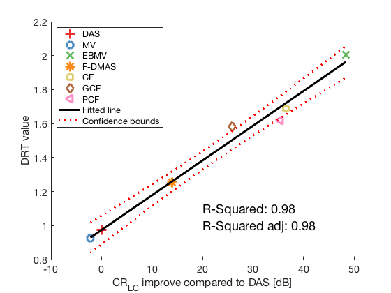
Plotting correlation plot between CR improvement and DRT with all 7 methods (excluding GLT)
lmd_sim_slope = fitlm(cr_improvement(1:7),DRT_value_exp(1:7))

lmd_sim_slope.Rsquared.Ordinary
lmd_sim_slope.Rsquared.Adjusted

f113 = figure(114);clf;hold all;
linespes = '+ox*sd<>';
for i = 1:length(image.all)-1
    plot(cr_improvement(i),DRT_value_exp(i),linespes(i),'Color',colors(i,:),'MarkerSize',10);
end
lmd_sim_slope.plot
hline = findobj(gcf, 'type', 'line');
set(hline,'LineWidth',3);
set(hline(3),'Color',[0 0 0]);
set(hline(3),'DisplayName','Fitted line');
title('')
xlabel('CR_{LC} improve compared to DAS [dB]','Interpreter', 'tex');
ylabel('DRT value');%ylim([-50 5]);
text(20,1.1,sprintf('R-Squared: %.2f',lmd_sim_slope.Rsquared.Ordinary),'FontSize',18);
text(20,1,sprintf('R-Squared adj: %.2f',lmd_sim_slope.Rsquared.Adjusted),'FontSize',18);
set(gca,'FontSize',14);
delete(hline(4));
legend();
hLegend = findobj(gcf, 'Type', 'Legend');
legend show
legend([{image.tags{1:7}} hLegend.String],'Location','nw');


saveas(f113,[ustb_path,filesep,'publications/DynamicRange/figures/experimental/correlation_experimental_withouth_GLT'],'eps2c')
lmd_sim_slope =


Linear regression model:
    y ~ 1 + x1

Estimated Coefficients:
                   Estimate       SE        tStat       pValue
                   ________    _________    ______    __________

    (Intercept)     0.97357     0.033048    29.459    8.4504e-07
    x1             0.020453    0.0011491      17.8    1.0272e-05


Number of observations: 7, Error degrees of freedom: 5
Root Mean Squared Error: 0.0543
R-squared: 0.984,  Adjusted R-Squared 0.981
F-statistic vs. constant model: 317, p-value = 1.03e-05

ans =

    0.9845


ans =

    0.9814
Save the data to a file to read parts of the results to be plotted with the simulated data
save([ustb_path,filesep,'publications/DynamicRange/','Experimental.mat'],'b_data_das','image','CR_signal_exp', ...
                        'CR_image_exp', 'CNR_signal_exp', 'CNR_image_exp','DRT_value_exp');