Create the figures from the simulated dynamic range phantom

For the publication Rindal, O. M. H., Austeng, A., Fatemi, A., & Rodriguez-Molares, A. (2019). The effect of dynamic range alterations in the estimation of contrast. Submitted to IEEE Transactions on Ultrasonics, Ferroelectrics, and Frequency Control.

NB! You need to run the create_figures_from_experimental.m first since we are using the stored experimental gradient values and contrast values to plot both the simulated and the experimental in the same plot.

Author: Ole Marius Hoel Rindal olemarius@olemarius.net 05.06.18 updated for revised version of manuscript 07.03.19

Load the data from the uff file
Print authorship and citation details for the dataset
DAS - Delay-And-Sum
GLT - Gray Level Transform
CF - Coherence Factor
PCF - Phase Coherence Factor
GCF - Generalized Coherence Factor
MV - Capon's Minimum Variance
F-DMAS - Filtered-Delay-Multiply-and-Sum
EBMV - Eigenspace Based Minimum Variance
Putting the dB images and the signal in a cell array
Plot the lateral and axial gradient together with the experimental lateral gradient
Plot the lateral line through the boxes
Calibrate images
Plot the lateral line through the boxes after calibration
Measure contrast and plot together with the experimental
Run Dynamic Range Test

Load the data from the uff file

clear all;
close all;
addpath([ustb_path,filesep,'publications',filesep,'DynamicRange',filesep,'functions',filesep])

filename = 'FieldII_STAI_dynamic_range.uff';
url='http://ustb.no/datasets/';      % if not found downloaded from here

% checks if the data is in your data path, and downloads it otherwise.
% The defaults data path is under USTB's folder, but you can change this
% by setting an environment variable with setenv(DATA_PATH,'the_path_you_want_to_use');
tools.download(filename, url, data_path);

channel_data = uff.channel_data();
channel_data.read([data_path,filesep,filename],'/channel_data');

b_data_das = uff.beamformed_data();
b_data_cf = uff.beamformed_data();
b_data_pcf = uff.beamformed_data();
b_data_gcf = uff.beamformed_data();
b_data_mv = uff.beamformed_data();
b_data_ebmv = uff.beamformed_data();
b_data_dmas = uff.beamformed_data();
b_data_weights = uff.beamformed_data();

b_data_das.read([data_path,filesep,filename],'/b_data_das');
b_data_cf.read([data_path,filesep,filename],'/b_data_cf');
b_data_pcf.read([data_path,filesep,filename],'/b_data_pcf');
b_data_gcf.read([data_path,filesep,filename],'/b_data_gcf');
b_data_mv.read([data_path,filesep,filename],'/b_data_mv');
b_data_ebmv.read([data_path,filesep,filename],'/b_data_ebmv');
b_data_dmas.read([data_path,filesep,filename],'/b_data_dmas');
b_data_weights.read([data_path,filesep,filename],'/b_data_weights');

weights = b_data_weights.get_image('none');

mkdir([ustb_path,filesep,'publications/DynamicRange/figures/simulation/']);
mkdir([ustb_path,filesep,'publications/DynamicRange/figures/simulation/gradient/']);
mkdir([ustb_path,filesep,'publications/DynamicRange/figures/simulation/calibrated/']);
mkdir([ustb_path,filesep,'publications/DynamicRange/figures/simulation/dynamic_range_test/']);

UFF: reading channel_data [uff.channel_data]
UFF: reading sequence [uff.wave] [====================] 100%
UFF: reading /b_data_das [uff.beamformed_data]
UFF: reading /b_data_cf [uff.beamformed_data]
UFF: reading /b_data_pcf [uff.beamformed_data]
UFF: reading /b_data_gcf [uff.beamformed_data]
UFF: reading /b_data_mv [uff.beamformed_data]
UFF: reading /b_data_ebmv [uff.beamformed_data]
UFF: reading /b_data_dmas [uff.beamformed_data]
UFF: reading /b_data_weights [uff.beamformed_data]
Warning: Directory already exists. 
Warning: Directory already exists. 
Warning: Directory already exists. 
Warning: Directory already exists.

Print authorship and citation details for the dataset

channel_data.print_authorship

Name: 		 v5 Simulated dynamic range phantom. Created with  
		 Field II. See the reference for details 
Reference: 	 Rindal, O. M. H., Austeng, A., Fatemi, A., &  
		 Rodriguez-Molares, A. (2018). The effect of  
		 dynamic range transformations in the estimation  
		 of contrast. Submitted to IEEE Transactions on  
		 Ultrasonics, Ferroelectrics, and Frequency  
		 Control. 
Author(s): 	 Ole Marius Hoel Rindal <omrindal@ifi.uio.no 
		 Alfonso Rodriguez-Molares <alfonso.r.molares@ntnu.no> 
Version: 	 1.0.1

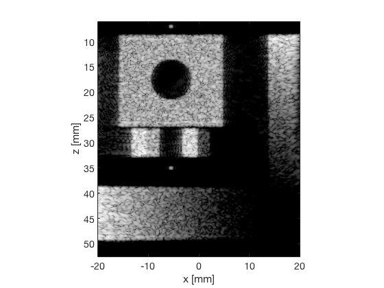
DAS - Delay-And-Sum

Create the individual images and the zoomed images on the boxes

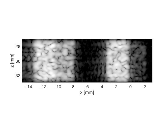
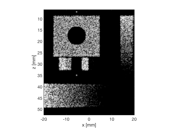
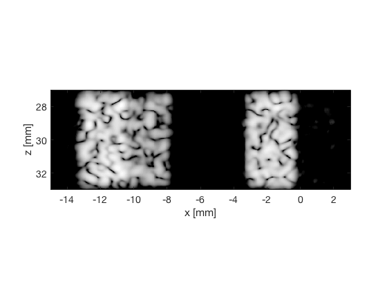
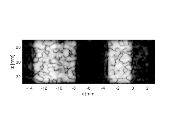
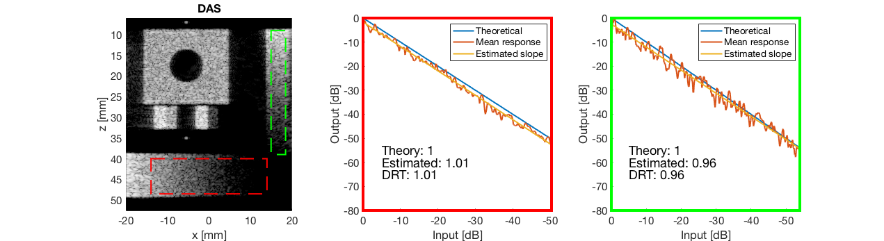
das_img = b_data_das.get_image('none').*weights;  % Compensation weighting
b_data_das.data = das_img(:); %Putting the weighted data back...
das_img = db(abs(das_img./max(das_img(:))));      % Normalize on max
f1 = figure(1);clf;
imagesc(b_data_das.scan.x_axis*1000,b_data_das.scan.z_axis*1000,das_img);
colormap gray;caxis([-60 0]);axis image;xlabel('x [mm]');ylabel('z [mm]');
set(gca,'FontSize',14);
saveas(f1,[ustb_path,filesep,'publications/DynamicRange/figures/simulation/DAS'],'eps2c')
saveas(f1,[ustb_path,filesep,'publications/DynamicRange/figures/simulation/DAS'],'png')
f2 = figure(2);clf;
imagesc(b_data_das.scan.x_axis*1000,b_data_das.scan.z_axis*1000,das_img);
colormap gray;caxis([-60 0]);axis image;xlabel('x [mm]');ylabel('z [mm]');
set(gca,'FontSize',14)
axis([-15 3 27 33]);
saveas(f2,[ustb_path,filesep,'publications/DynamicRange/figures/simulation/DAS_zoomed'],'eps2c')

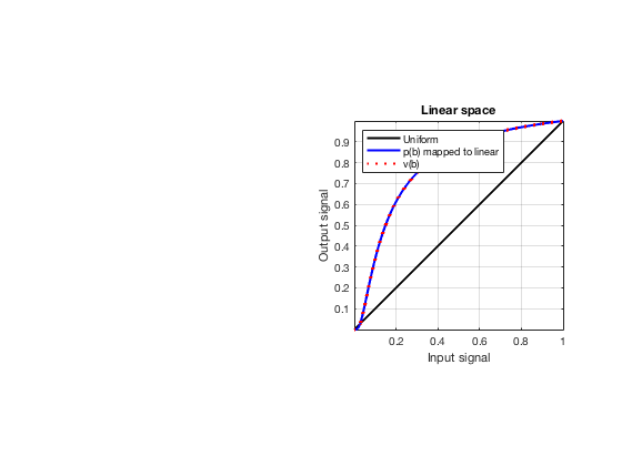
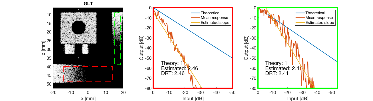
GLT - Gray Level Transform

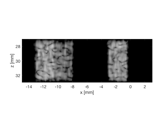
glt_s = postprocess.scurve_gray_level_transform();

glt_s.a = 0.12;
glt_s.b = -40;
glt_s.c = 0.008;

glt_s.plot_functions = 1;
glt_s.input = b_data_das;
glt_s.scan = b_data_das.scan;
b_data_glt = glt_s.go();

glt_img = b_data_glt.get_image('none');  % Compensation weighting
b_data_glt.data = glt_img(:);
glt_img = db(abs(glt_img./max(glt_img(:)))+eps);      % Normalize on max
f100 = figure(100);clf;
imagesc(b_data_das.scan.x_axis*1000,b_data_das.scan.z_axis*1000,glt_img);
colormap gray;caxis([-60 0]);axis image;xlabel('x [mm]');ylabel('z [mm]');
set(gca,'FontSize',14)
saveas(f100,[ustb_path,filesep,'publications/DynamicRange/figures/simulation/GLT'],'eps2c')

f101 = figure(101);clf;
imagesc(b_data_das.scan.x_axis*1000,b_data_das.scan.z_axis*1000,glt_img);
colormap gray;caxis([-60 0]);axis image;xlabel('x [mm]');ylabel('z [mm]');
set(gca,'FontSize',14)
axis([-15 3 27 33]);
saveas(f101,[ustb_path,filesep,'publications/DynamicRange/figures/simulation/GLT_zoomed'],'eps2c')

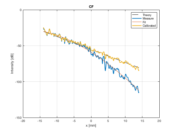
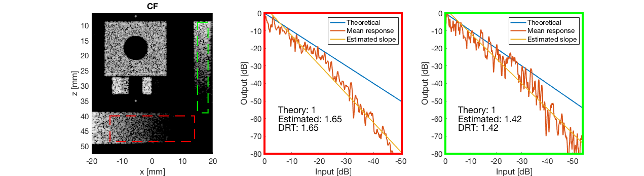
CF - Coherence Factor

cf_img = b_data_cf.get_image('none').*weights;
b_data_cf.data = cf_img(:);
cf_img = db(abs(cf_img./max(cf_img(:))));                 % Normalize on max
f2 = figure(2);
imagesc(b_data_das.scan.x_axis*1000,b_data_das.scan.z_axis*1000,cf_img);
colormap gray;caxis([-60 0]);axis image;xlabel('x [mm]');ylabel('z [mm]');
set(gca,'FontSize',14)
saveas(f2,[ustb_path,filesep,'publications/DynamicRange/figures/simulation/CF'],'eps2c')
f22 = figure(22);
imagesc(b_data_das.scan.x_axis*1000,b_data_das.scan.z_axis*1000,cf_img);
colormap gray;caxis([-60 0]);axis image;xlabel('x [mm]');ylabel('z [mm]');
set(gca,'FontSize',14)
axis([-15 3 27 33]);
saveas(f22,[ustb_path,filesep,'publications/DynamicRange/figures/simulation/CF_zoomed'],'eps2c')

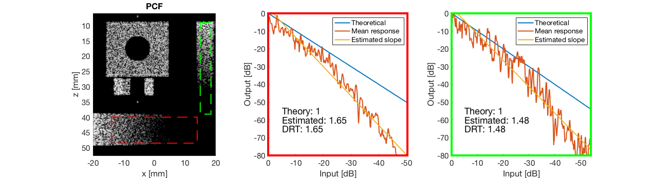
PCF - Phase Coherence Factor

pcf_img = b_data_pcf.get_image('none').*weights;
b_data_pcf.data = pcf_img(:);
b_data_pcf.data(isinf(b_data_pcf.data)) = eps;
b_data_pcf.data(b_data_pcf.data==0) = eps;
pcf_img(isinf(pcf_img)) = eps;
pcf_img(pcf_img==0) = eps;
pcf_img = db(abs(pcf_img./max(pcf_img(:)))+eps);
f3 = figure(3);clf;
imagesc(b_data_das.scan.x_axis*1000,b_data_das.scan.z_axis*1000,pcf_img);
colormap gray;caxis([-60 0]);axis image;xlabel('x [mm]');ylabel('z [mm]');
set(gca,'FontSize',14)
saveas(f3,[ustb_path,filesep,'publications/DynamicRange/figures/simulation/PCF'],'eps2c')
f33 = figure(33);clf;
imagesc(b_data_das.scan.x_axis*1000,b_data_das.scan.z_axis*1000,pcf_img);
colormap gray;caxis([-60 0]);axis image;xlabel('x [mm]');ylabel('z [mm]');
set(gca,'FontSize',14)
axis([-15 3 27 33]);
saveas(f33,[ustb_path,filesep,'publications/DynamicRange/figures/simulation/PCF_zoomed'],'eps2c')

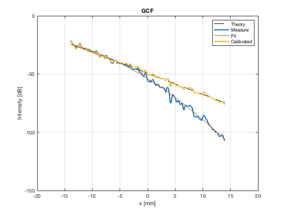
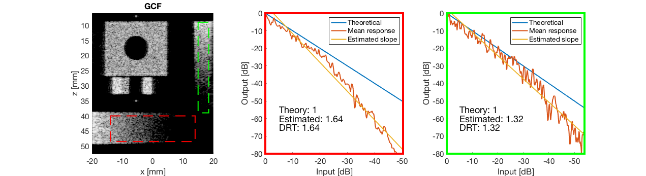
GCF - Generalized Coherence Factor

gcf_img = b_data_gcf.get_image('none').*weights;
b_data_gcf.data = gcf_img(:);
gcf_img = db(abs(gcf_img./max(gcf_img(:))));
f4 = figure(4);clf;
imagesc(b_data_das.scan.x_axis*1000,b_data_das.scan.z_axis*1000,gcf_img);
colormap gray;caxis([-60 0]);axis image;xlabel('x [mm]');ylabel('z [mm]');
set(gca,'FontSize',14)
saveas(f4,[ustb_path,filesep,'publications/DynamicRange/figures/simulation/GCF'],'eps2c')
f44 = figure(44);
imagesc(b_data_das.scan.x_axis*1000,b_data_das.scan.z_axis*1000,gcf_img);
colormap gray;caxis([-60 0]);axis image;xlabel('x [mm]');ylabel('z [mm]');
set(gca,'FontSize',14)
axis([-15 3 27 33]);
saveas(f44,[ustb_path,filesep,'publications/DynamicRange/figures/simulation/GCF_zoomed'],'eps2c')

MV - Capon's Minimum Variance

mv_img = b_data_mv.get_image('none').*weights;
b_data_mv.data = mv_img(:);
mv_img = db(abs(mv_img./max(mv_img(:))));
f6 = figure(6);clf;
imagesc(b_data_das.scan.x_axis*1000,b_data_das.scan.z_axis*1000,mv_img);
colormap gray;caxis([-60 0]);axis image;xlabel('x [mm]');ylabel('z [mm]');
set(gca,'FontSize',14)
saveas(f6,[ustb_path,filesep,'publications/DynamicRange/figures/simulation/MV'],'eps2c')
f66 = figure(66);clf;
imagesc(b_data_das.scan.x_axis*1000,b_data_das.scan.z_axis*1000,mv_img);
colormap gray;caxis([-60 0]);axis image;xlabel('x [mm]');ylabel('z [mm]');
set(gca,'FontSize',14)
axis([-15 3 27 33]);
saveas(f66,[ustb_path,filesep,'publications/DynamicRange/figures/simulation/MV_zoomed'],'eps2c')

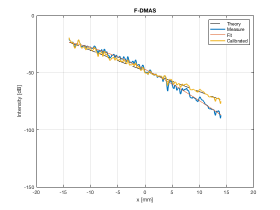
F-DMAS - Filtered-Delay-Multiply-and-Sum

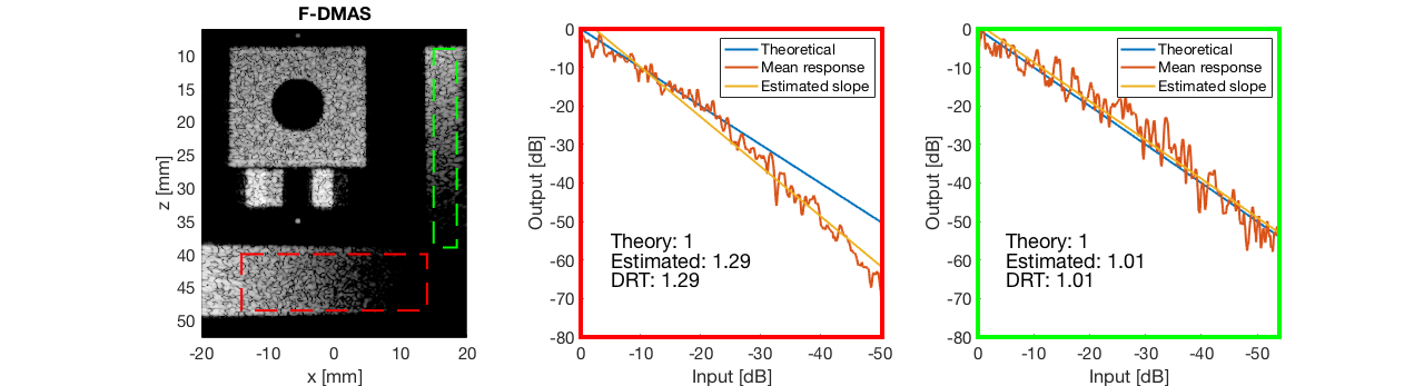
dmas_img = b_data_dmas.get_image('none').*weights;
b_data_dmas.data = dmas_img(:);
dmas_img = db(abs(dmas_img./max(dmas_img(:))));
f7 = figure(7);clf;
imagesc(b_data_das.scan.x_axis*1000,b_data_das.scan.z_axis*1000,dmas_img);
colormap gray;caxis([-60 0]);axis image;xlabel('x [mm]');ylabel('z [mm]');
set(gca,'FontSize',14)
saveas(f7,[ustb_path,filesep,'publications/DynamicRange/figures/simulation/DMAS'],'eps2c')
f77 = figure(77);clf;
imagesc(b_data_das.scan.x_axis*1000,b_data_das.scan.z_axis*1000,dmas_img);
colormap gray;caxis([-60 0]);axis image;xlabel('x [mm]');ylabel('z [mm]');
set(gca,'FontSize',14)
axis([-15 3 27 33]);
saveas(f77,[ustb_path,filesep,'publications/DynamicRange/figures/simulation/DMAS_zoomed'],'eps2c')

EBMV - Eigenspace Based Minimum Variance

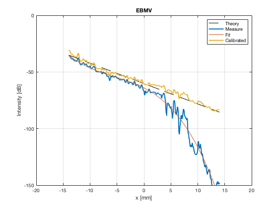
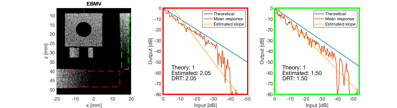
ebmv_img = b_data_ebmv.get_image('none').*weights;
b_data_ebmv.data = ebmv_img(:);
ebmv_img = db(abs(ebmv_img./max(ebmv_img(:))));
f8 = figure(8);clf;
imagesc(b_data_das.scan.x_axis*1000,b_data_das.scan.z_axis*1000,ebmv_img);
colormap gray;caxis([-60 0]);axis image;xlabel('x [mm]');ylabel('z [mm]');
set(gca,'FontSize',14)
saveas(f8,[ustb_path,filesep,'publications/DynamicRange/figures/simulation/EBMV'],'eps2c')
f88 = figure(88);clf;
imagesc(b_data_das.scan.x_axis*1000,b_data_das.scan.z_axis*1000,ebmv_img);
colormap gray;caxis([-60 0]);axis image;xlabel('x [mm]');ylabel('z [mm]');
set(gca,'FontSize',14)
axis([-15 3 27 33]);
saveas(f88,[ustb_path,filesep,'publications/DynamicRange/figures/simulation/EBMV_zoomed'],'eps2c')

Putting the dB images and the signal in a cell array

addpath([ustb_path,'/publications/DynamicRange/functions']);
image.all{1} = das_img;
image.all_signal{1} = double(b_data_das.get_image('none'));
image.all_signal{1} = (image.all_signal{1}./max(image.all_signal{1}(:)));
image.tags{1} = 'DAS';
image.all{2} = mv_img;
image.all_signal{2} = double(b_data_mv.get_image('none'));
image.all_signal{2} = (image.all_signal{2}./max(image.all_signal{2}(:)));
image.tags{2} = 'MV';
image.all{3} = ebmv_img;
image.all_signal{3} = double(b_data_ebmv.get_image('none'));
image.all_signal{3} = (image.all_signal{3}./max(image.all_signal{3}(:)));
image.tags{3} = 'EBMV';
image.all{4} = dmas_img;
image.all_signal{4} = double(b_data_dmas.get_image('none'));
image.all_signal{4} = (image.all_signal{4}./max(image.all_signal{4}(:)));
image.tags{4} = 'F-DMAS';
image.all{5} = cf_img;
image.all_signal{5} = double(b_data_cf.get_image('none'));
image.all_signal{5} = (image.all_signal{5}./max(image.all_signal{5}(:)));
image.tags{5} = 'CF';
image.all{6} = gcf_img;
image.all_signal{6} = double(b_data_gcf.get_image('none'));
image.all_signal{6} = (image.all_signal{6}./max(image.all_signal{6}(:)));
image.tags{6} = 'GCF';
image.all{7} = pcf_img;
image.all_signal{7} = double(b_data_pcf.get_image('none'));
image.all_signal{7}(isinf(image.all_signal{7})) = eps;
image.all_signal{7} = (image.all_signal{7}./max(image.all_signal{7}(:)));
image.tags{7} = 'PCF';
image.all{8} = glt_img;
image.all_signal{8} = double(b_data_glt.get_image('none'));
image.all_signal{8} = (image.all_signal{8}./max(image.all_signal{8}(:)));
image.tags{8} = 'GLT';

% Using "linspecer" colors
colors=    [0.9047    0.1918    0.1988; ...
            0.2941    0.5447    0.7494; ...
            0.3718    0.7176    0.3612; ...
            1.0000    0.5482    0.1000; ...
            0.8650    0.8110    0.4330; ...
            0.6859    0.4035    0.2412; ...
            0.9718    0.5553    0.7741; ...
            0.6400    0.6400    0.6400];

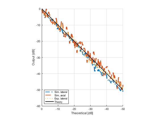
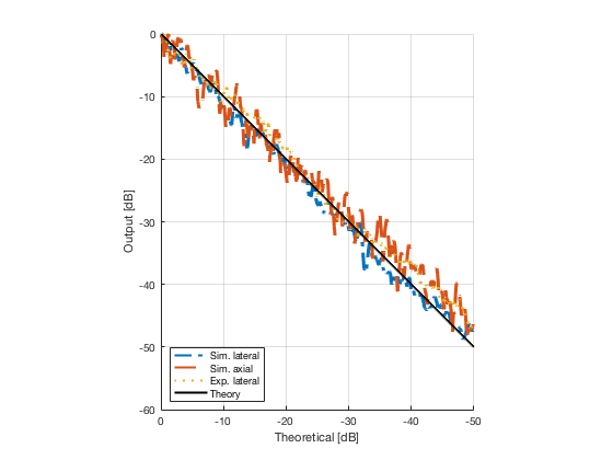
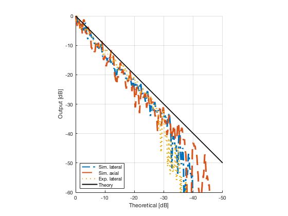
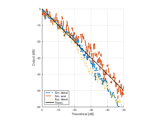
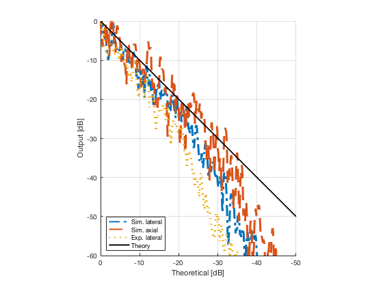
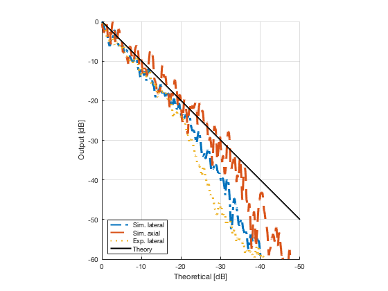
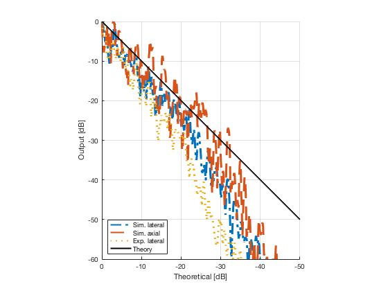
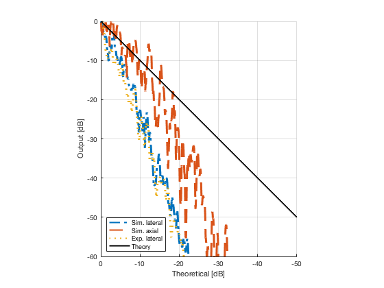
Plot the lateral and axial gradient together with the experimental lateral gradient

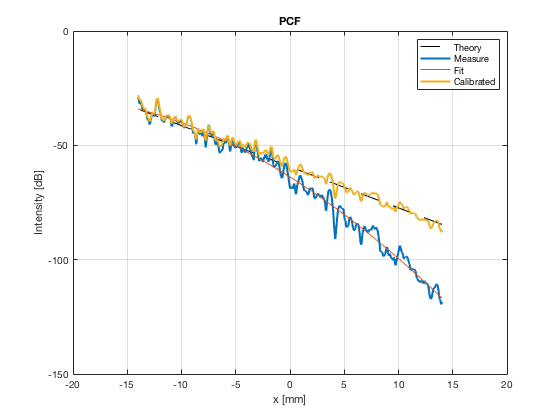
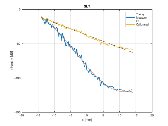
image_experimental = load([ustb_path,'/publications/DynamicRange/','Experimental.mat'],'image');
image_experimental = image_experimental.image;
b_data_das_exp = load([ustb_path,'/publications/DynamicRange/','Experimental.mat'],'b_data_das');
b_data_das_exp = b_data_das_exp.b_data_das;

x_axis_grad_start = 14;

[meanLinesLateralExp,~] = getMeanLateralLines(b_data_das_exp,image_experimental,39,48.5,-x_axis_grad_start,x_axis_grad_start);

gradient = -1.8;

mask_lateral_exp=abs(b_data_das_exp.scan.x_axis)<x_axis_grad_start*10^-3;
%theory_lateral_exp=-40*(b_data_das_exp.scan.x_axis(mask_lateral_exp)+x_axis_grad_start*10^-3)/24.1e-3;
theory_lateral_exp = (gradient*(b_data_das_exp.scan.x_axis(mask_lateral_exp)+x_axis_grad_start*10^-3))*10^3;

[meanLinesLateral,x_axis] = getMeanLateralLines(b_data_das,image,39,48.5,-x_axis_grad_start,x_axis_grad_start);
mask_lateral=abs(b_data_das.scan.x_axis)<x_axis_grad_start*10^-3;
theory_lateral = (gradient*(b_data_das.scan.x_axis(mask_lateral)+x_axis_grad_start*10^-3))*10^3;

[meanLines_axial,z_axis] = getMeanAxialLines(b_data_das,image,10,38,15,18.5);
mask_axial= b_data_das.scan.z_axis<38e-3 & b_data_das.scan.z_axis>10e-3;
theory_axial = (gradient*(b_data_das.scan.z_axis(mask_axial)-10e-3))*10^3;

for i = 1:length(image.all)
    f88 = figure(8888+i);clf;hold all;
    plot(theory_lateral,meanLinesLateral.all{i}-max(meanLinesLateral.all{i}),'LineStyle','-.','Linewidth',2,'DisplayName','Sim. lateral');
    plot(theory_axial,meanLines_axial.all{i}-max(meanLines_axial.all{i}),'Linestyle','--','Linewidth',2,'DisplayName','Sim. axial');
    plot(theory_lateral_exp,meanLinesLateralExp.all{i}-max(meanLinesLateralExp.all{i}),'Linestyle',':','Linewidth',2,'DisplayName','Exp. lateral');
    plot(theory_lateral,theory_lateral,'LineStyle','-','Linewidth',2,'Color','k','DisplayName','Theory');
    set(gca, 'XDir','reverse');%title(image.tags{i});
    axis image
    legend('show','Location','sw');
    ylim([-60 0])
    xlim([-50 0])
    grid on
    xlabel('Theoretical [dB]');
    ylabel('Output [dB]');
    saveas(f88,[ustb_path,filesep,'publications/DynamicRange/figures/simulation/gradient/',image.tags{i}],'eps2c')
    %saveas(f88,[ustb_path,filesep,'publications/DynamicRange/figures/simulation/gradient/',image.tags{i}],'png')
end

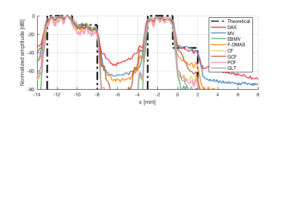
Plot the lateral line through the boxes

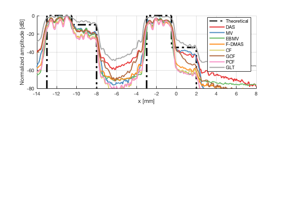
[meanLines,x_axis] = getMeanLateralLines(b_data_das,image,27.5,32.5,b_data_das.scan.x(1)*10^3,b_data_das.scan.x(end)*10^3);
theoretical = [-100 ones(1,255)*0 ones(1,255)*-10 -100 ones(1,256)*-100 ones(1,256)*-100 -100 ones(1,255)*0 ones(1,255)*-35 -100];
x_axis_theoretical = linspace(-13,2,1536);

f89 = figure(89);clf;hold all;
subplot(211);hold on;
plot(x_axis_theoretical,theoretical,'LineStyle','-.','Linewidth',2,'DisplayName','Theoretical','Color',[0 0 0]);
plot(x_axis,meanLines.all{1}-max(meanLines.all{1}),'Linewidth',2,'DisplayName',image.tags{1},'Color',colors(1,:));
plot(x_axis,meanLines.all{2}-max(meanLines.all{2}),'Linewidth',2,'DisplayName',image.tags{2},'Color',colors(2,:));
plot(x_axis,meanLines.all{3}-max(meanLines.all{3}),'Linewidth',2,'DisplayName',image.tags{3},'Color',colors(3,:));
plot(x_axis,meanLines.all{4}-max(meanLines.all{4}),'Linewidth',2,'DisplayName',image.tags{4},'Color',colors(4,:));
plot(x_axis,meanLines.all{5}-max(meanLines.all{5}),'Linewidth',2,'DisplayName',image.tags{5},'Color',colors(5,:));
plot(x_axis,meanLines.all{6}-max(meanLines.all{6}),'Linewidth',2,'DisplayName',image.tags{6},'Color',colors(6,:));
plot(x_axis,meanLines.all{7}-max(meanLines.all{7}),'Linewidth',2,'DisplayName',image.tags{7},'Color',colors(7,:));
plot(x_axis,meanLines.all{8}-max(meanLines.all{8}),'Linewidth',2,'DisplayName',image.tags{8},'Color',colors(8,:));
ylim([-80 0]);
xlim([-14 8]);
legend('Location','best'); grid on;
ylabel('Normalized amplitude [dB]');
xlabel('x [mm]');

saveas(f89,[ustb_path,filesep,'publications/DynamicRange/figures/simulation/boxes'],'eps2c')

Calibrate images

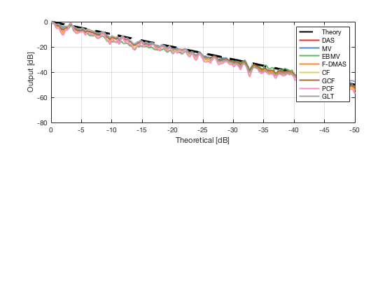
[image_calibrated_on_theoretical] = calibrateImage_on_theoretical(b_data_das,image,40,48.5,-14,14,3,1.8,colors);

x_axis_grad_start = 14;
mask_lateral=abs(b_data_das.scan.x_axis)<x_axis_grad_start*10^-3;
theory_lateral = (-1.8*(b_data_das.scan.x_axis(mask_lateral)+x_axis_grad_start*10^-3))*10^3;

[meanLines_calibrated,~] = getMeanLateralLines(b_data_das,image_calibrated_on_theoretical,39,48.5,-x_axis_grad_start,x_axis_grad_start);

f10 = figure(77);clf;hold all;
subplot(211);
plot(theory_lateral,theory_lateral,'k--','DisplayName','Theory','linewidth',2); hold on; grid on;
for i = 1:length(image_calibrated_on_theoretical.all)
    plot(theory_lateral,meanLines_calibrated.all{i}-max(meanLines_calibrated.all{i}),'linewidth',2,'DisplayName',image.tags{i},'Color',colors(i,:));
end
xlabel('Theoretical [dB]');
ylabel('Output [dB]');
set(gca, 'XDir','reverse');
xlim([-50 0])
ylim([-80 0])
legend show
saveas(f10,[ustb_path,filesep,'publications/DynamicRange/figures/simulation/calibrated/calibrated_all_curves_on_theoretical'],'eps2c')

Plot the lateral line through the boxes after calibration

[meanLines,x_axis] = getMeanLateralLines(b_data_das,image_calibrated_on_theoretical,27.5,32.5,b_data_das.scan.x(1)*10^3,b_data_das.scan.x(end)*10^3);
theoretical = [-100 ones(1,255)*0 ones(1,255)*-10 -100 ones(1,256)*-100 ones(1,256)*-100 -100 ones(1,255)*0 ones(1,255)*-35 -100];
x_axis_theoretical = linspace(-13,2,1536);

f89 = figure(90);clf;hold all;
subplot(211);hold on;
plot(x_axis_theoretical,theoretical,'LineStyle','-.','Linewidth',2,'DisplayName','Theoretical','Color',[0 0 0]);
plot(x_axis,meanLines.all{1}-max(meanLines.all{1}),'Linewidth',2,'DisplayName',image.tags{1},'Color',colors(1,:));
plot(x_axis,meanLines.all{2}-max(meanLines.all{2}),'Linewidth',2,'DisplayName',image.tags{2},'Color',colors(2,:));
plot(x_axis,meanLines.all{3}-max(meanLines.all{3}),'Linewidth',2,'DisplayName',image.tags{3},'Color',colors(3,:));
plot(x_axis,meanLines.all{4}-max(meanLines.all{4}),'Linewidth',2,'DisplayName',image.tags{4},'Color',colors(4,:));
plot(x_axis,meanLines.all{5}-max(meanLines.all{5}),'Linewidth',2,'DisplayName',image.tags{5},'Color',colors(5,:));
plot(x_axis,meanLines.all{6}-max(meanLines.all{6}),'Linewidth',2,'DisplayName',image.tags{6},'Color',colors(6,:));
plot(x_axis,meanLines.all{7}-max(meanLines.all{7}),'Linewidth',2,'DisplayName',image.tags{7},'Color',colors(7,:));
plot(x_axis,meanLines.all{8}-max(meanLines.all{8}),'Linewidth',2,'DisplayName',image.tags{8},'Color',colors(8,:));
ylim([-80 0]);
xlim([-14 8]);
legend('Location','best'); grid on;
ylabel('Normalized amplitude [dB]');
xlabel('x [mm]');

saveas(f89,[ustb_path,filesep,'publications/DynamicRange/figures/simulation/calibrated/boxes_calibrated_lines_on_theoretical'],'eps2c')
saveas(f89,[ustb_path,filesep,'publications/DynamicRange/figures/simulation/calibrated/boxes_calibrated_lines_on_theoretical'],'png')

Measure contrast and plot together with the experimental

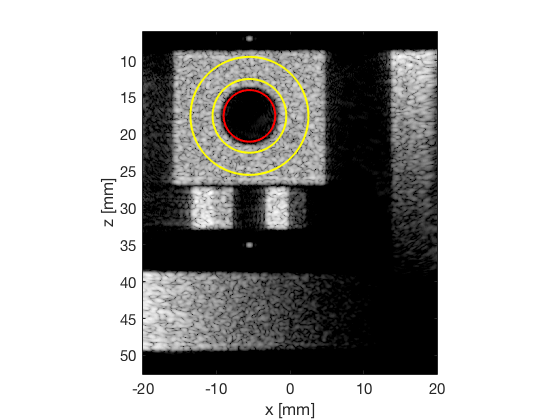
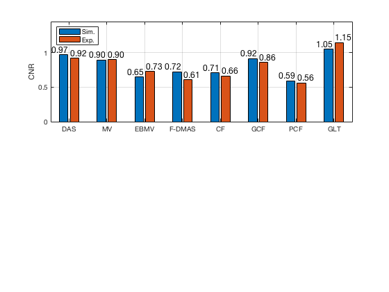
[CR_signal_sim, CR_signal_dagger, CR_image_sim, CNR_signal_sim, CNR_image_sim] = measureContrast(b_data_das,image,-5.5,17.5,3.5,5,8,[ustb_path,filesep,'publications/DynamicRange/figures/simulation/DAS_cyst_indicated']);

load('Experimental.mat','CR_signal_exp','CNR_signal_exp','CR_image_exp','CNR_image_exp');

f9 = figure;
subplot(211);
bar([10*log10(CR_signal_sim)' 10*log10(CR_signal_exp)'])
set(gca,'XTick',linspace(1,length(image.tags),length(image.tags)))
set(gca,'XTickLabel',image.tags)
ylabel('CR [dB]');
x_pos = [0.8 1.8 2.8 3.8 4.8 5.8 6.8 7.8];
text(x_pos,double(10*log10(CR_signal_sim(:))),num2str(round(10*log10(CR_signal_sim(:))),'%d'),...
    'HorizontalAlignment','center',...
    'VerticalAlignment','bottom',...
    'FontSize',12)
x_pos = [1.2 2.2 3.2 4.2 5.2 6.2 7.2 8.2];
text(x_pos,double(10*log10(CR_signal_exp(:))),num2str(round(10*log10(CR_signal_exp(:))),'%d'),...
    'HorizontalAlignment','center',...
    'VerticalAlignment','bottom',...
    'FontSize',12)
set(gca,'Ydir','reverse')
legend('Sim.','Exp.','Location','nw')
grid on

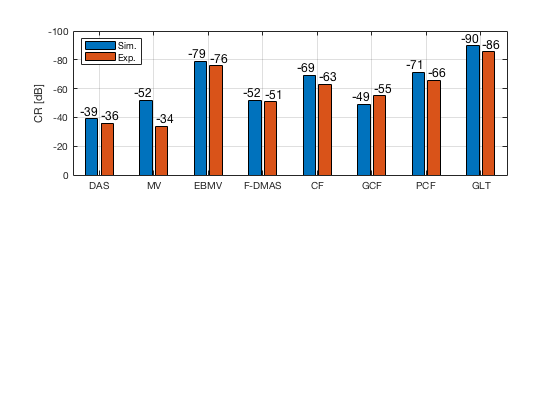
saveas(f9,[ustb_path,filesep,'publications/DynamicRange/figures/simulation/CR'],'eps2c')

f90 = figure;
subplot(212);
bar([CR_image_sim' CR_image_exp'])
set(gca,'XTick',linspace(1,length(image.tags),length(image.tags)))
set(gca,'XTickLabel',image.tags)
ylabel('CR_{LC} [dB]');
x_pos = [0.8 1.8 2.8 3.8 4.8 5.8 6.8 7.8];
text(x_pos,double(CR_image_sim(:)),num2str(round(CR_image_sim(:)),'%d'),...
    'HorizontalAlignment','center',...
    'VerticalAlignment','bottom',...
    'FontSize',12)
x_pos = [1.2 2.2 3.2 4.2 5.2 6.2 7.2 8.2];
text(x_pos,double(CR_image_exp(:)),num2str(round(CR_image_exp(:)),'%d'),...
    'HorizontalAlignment','center',...
    'VerticalAlignment','bottom',...
    'FontSize',12)
ylim([0 125])
legend('Sim.','Exp.','Location','nw')
grid on

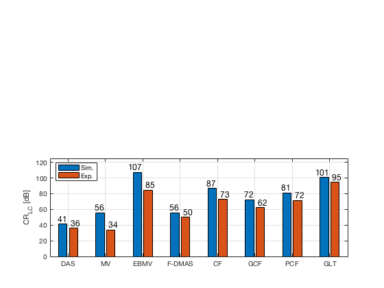
saveas(f90,[ustb_path,filesep,'publications/DynamicRange/figures/simulation/CR_LC'],'eps2c')

f77 = figure(77);clf;
subplot(211);
bar([CNR_signal_sim' CNR_signal_exp'])
set(gca,'XTick',linspace(1,length(image.tags),length(image.tags)))
set(gca,'XTickLabel',image.tags)
ylabel('CNR');
x_pos = [0.75 1.75 2.75 3.75 4.75 5.75 6.75 7.75];
text(x_pos,double(CNR_signal_sim(:)),num2str((CNR_signal_sim(:)),'%.2f'),...
    'HorizontalAlignment','center',...
    'VerticalAlignment','bottom',...
    'FontSize',12)
x_pos = [1.25 2.25 3.25 4.25 5.25 6.25 7.25 8.25];
text(x_pos,double(CNR_signal_exp(:)),num2str((CNR_signal_exp(:)),'%.2f'),...
    'HorizontalAlignment','center',...
    'VerticalAlignment','bottom',...
    'FontSize',12)
ylim([0 1.45])
legend('Sim.','Exp.','Location','nw')
grid on

saveas(f77,[ustb_path,filesep,'publications/DynamicRange/figures/simulation/CNR'],'eps2c')

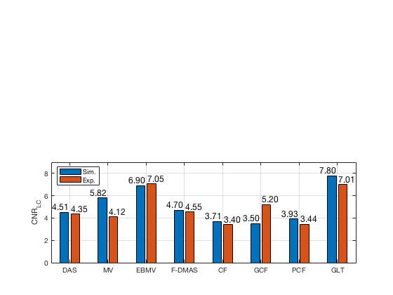
f78 = figure(78);clf;
subplot(212);
bar([CNR_image_sim' CNR_image_exp'])
set(gca,'XTick',linspace(1,length(image.tags),length(image.tags)))
set(gca,'XTickLabel',image.tags)
ylabel('CNR_{LC}');
x_pos = [0.75 1.75 2.75 3.75 4.75 5.75 6.75 7.75];
text(x_pos,double(CNR_image_sim(:)),num2str((CNR_image_sim(:)),'%.2f'),...
    'HorizontalAlignment','center',...
    'VerticalAlignment','bottom',...
    'FontSize',12)
x_pos = [1.25 2.25 3.25 4.25 5.25 6.25 7.25 8.25];
text(x_pos,double(CNR_image_exp(:)),num2str((CNR_image_exp(:)),'%.2f'),...
    'HorizontalAlignment','center',...
    'VerticalAlignment','bottom',...
    'FontSize',12)
legend('Sim.','Exp.','Location','nw')
grid on
ylim([0 9])

saveas(f78,[ustb_path,filesep,'publications/DynamicRange/figures/simulation/CNR_LC'],'eps2c')

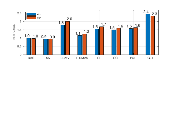
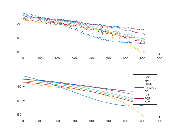
Run Dynamic Range Test

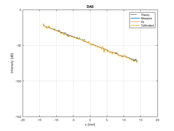
diff{1} = tools.dynamic_range_test(channel_data,b_data_das,'DAS');
set(gcf,'Position',[7 222 1271 347]);
saveas(gcf,[ustb_path,filesep,'publications/DynamicRange/figures/simulation/dynamic_range_test/','DAS'],'eps2c');
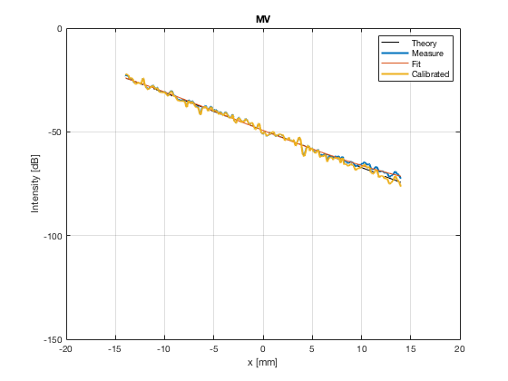
diff{2} = tools.dynamic_range_test(channel_data,b_data_mv,'MV');
set(gcf,'Position',[7 222 1271 347]);
saveas(gcf,[ustb_path,filesep,'publications/DynamicRange/figures/simulation/dynamic_range_test/','MV'],'eps2c');
diff{3} = tools.dynamic_range_test(channel_data,b_data_ebmv,'EBMV');
set(gcf,'Position',[7 222 1271 347]);
saveas(gcf,[ustb_path,filesep,'publications/DynamicRange/figures/simulation/dynamic_range_test/','EBMV'],'eps2c');
diff{4} = tools.dynamic_range_test(channel_data,b_data_dmas,'F-DMAS');
set(gcf,'Position',[7 222 1271 347]);
saveas(gcf,[ustb_path,filesep,'publications/DynamicRange/figures/simulation/dynamic_range_test/','F-DMAS'],'eps2c');
diff{5} = tools.dynamic_range_test(channel_data,b_data_cf,'CF');
set(gcf,'Position',[7 222 1271 347]);
saveas(gcf,[ustb_path,filesep,'publications/DynamicRange/figures/simulation/dynamic_range_test/','CF'],'eps2c');
diff{6} = tools.dynamic_range_test(channel_data,b_data_gcf,'GCF');
set(gcf,'Position',[7 222 1271 347]);
saveas(gcf,[ustb_path,filesep,'publications/DynamicRange/figures/simulation/dynamic_range_test/','GCF'],'eps2c');
diff{7} = tools.dynamic_range_test(channel_data,b_data_pcf,'PCF');
set(gcf,'Position',[7 222 1271 347]);
saveas(gcf,[ustb_path,filesep,'publications/DynamicRange/figures/simulation/dynamic_range_test/','PCF'],'eps2c');
diff{8} = tools.dynamic_range_test(channel_data,b_data_glt,'GLT');
set(gcf,'Position',[7 222 1271 347]);
saveas(gcf,[ustb_path,filesep,'publications/DynamicRange/figures/simulation/dynamic_range_test/','GLT'],'eps2c');

for i = 1:length(image.tags)
    DRT_value(i) = (mean(diff{i}));
end

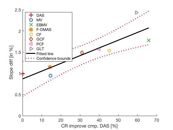
cr_improvement = CR_image_sim - CR_image_sim(1);

lmd_sim_slope = fitlm(cr_improvement(1:8),DRT_value(1:8))

lmd_sim_slope.Rsquared.Ordinary
lmd_sim_slope.Rsquared.Adjusted

f113 = figure(114);clf;hold all;
linespes = '+ox*sd<>';
for i = 1:length(image.all)
    plot(cr_improvement(i),DRT_value(i),linespes(i),'Color',colors(i,:),'MarkerSize',10);
end
lmd_sim_slope.plot
hline = findobj(gcf, 'type', 'line');
set(hline,'LineWidth',3);
set(hline(3),'Color',[0 0 0]);
set(hline(3),'DisplayName','Fitted line');
title('')
xlabel('CR improve cmp. DAS [%]');%xlim([-5 75]);
ylabel('Slope diff [in %]');%ylim([-50 5]);
text(80,10,sprintf('R-Squared: %.2f',lmd_sim_slope.Rsquared.Ordinary),'FontSize',18);
text(80,0,sprintf('R-Squared adj: %.2f',lmd_sim_slope.Rsquared.Adjusted),'FontSize',18);
set(gca,'FontSize',14);
delete(hline(4));
legend();
hLegend = findobj(gcf, 'Type', 'Legend');
legend show
legend([{image.tags{1:8}} hLegend.String],'Location','nw');

saveas(f113,[ustb_path,filesep,'publications/DynamicRange/figures/simulation/correlation_simulation'],'eps2c')

lmd_sim_slope = 


Linear regression model:
    y ~ 1 + x1

Estimated Coefficients:
                   Estimate       SE       tStat      pValue  
                   ________    ________    ______    _________

    (Intercept)     0.86838     0.16773    5.1773    0.0020598
    x1             0.018225    0.004179     4.361    0.0047651


Number of observations: 8, Error degrees of freedom: 6
Root Mean Squared Error: 0.256
R-squared: 0.76,  Adjusted R-Squared 0.72
F-statistic vs. constant model: 19, p-value = 0.00477

ans =

    0.7602


ans =

    0.7202

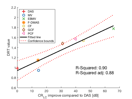
lmd_sim_slope = fitlm(cr_improvement(1:7),DRT_value(1:7))

lmd_sim_slope.Rsquared.Ordinary
lmd_sim_slope.Rsquared.Adjusted

f113 = figure(114);clf;hold all;
linespes = '+ox*sd<>';
for i = 1:length(image.all)-1
    plot(cr_improvement(i),DRT_value(i),linespes(i),'Color',colors(i,:),'MarkerSize',10);
end
lmd_sim_slope.plot
hline = findobj(gcf, 'type', 'line');
set(hline,'LineWidth',3);
set(hline(3),'Color',[0 0 0]);
set(hline(3),'DisplayName','Fitted line');
title('')
xlabel('CR_{LC} improve compared to DAS [dB]','Interpreter', 'tex');
ylabel('DRT value');
text(40,1,sprintf('R-Squared: %.2f',lmd_sim_slope.Rsquared.Ordinary),'FontSize',18);
text(40,0.9,sprintf('R-Squared adj: %.2f',lmd_sim_slope.Rsquared.Adjusted),'FontSize',18);
set(gca,'FontSize',14);
delete(hline(4));
legend();
hLegend = findobj(gcf, 'Type', 'Legend');
legend show
legend([{image.tags{1:7}} hLegend.String],'Location','nw');


saveas(f113,[ustb_path,filesep,'publications/DynamicRange/figures/simulation/correlation_simulation_without_glt'],'eps2c')

lmd_sim_slope = 


Linear regression model:
    y ~ 1 + x1

Estimated Coefficients:
                   Estimate       SE        tStat       pValue  
                   ________    _________    ______    __________

    (Intercept)     0.94049     0.075572    12.445    5.9395e-05
    x1             0.013554    0.0020665    6.5588      0.001235


Number of observations: 7, Error degrees of freedom: 5
Root Mean Squared Error: 0.113
R-squared: 0.896,  Adjusted R-Squared 0.875
F-statistic vs. constant model: 43, p-value = 0.00123

ans =

    0.8959


ans =

    0.8750

load([ustb_path,'/publications/DynamicRange/','Experimental.mat'],'DRT_value_exp');
f10 = figure(10);clf;
subplot(211);
bar([DRT_value' DRT_value_exp'])
set(gca,'XTick',linspace(1,length(image.tags),length(image.tags)))
set(gca,'XTickLabel',image.tags)
ylabel('DRT value');
legend('Location','nw','sim.','exp.')
x_pos = [0.75 1.25 1.75 2.25 2.75 3.25 3.75 4.25 4.75 5.25 5.75 6.25 6.75 7.25 7.75 8.25];
DRT_value_all = [];
for i = 1:length(DRT_value_exp)
    DRT_value_all = [DRT_value_all; DRT_value(i); DRT_value_exp(i)];
end
text(x_pos,double(DRT_value_all),num2str(DRT_value_all(:),'%0.1f'),...
    'HorizontalAlignment','center',...
    'VerticalAlignment','bottom',...
    'FontSize',12)
grid on;
ylim([0 2.7])

saveas(f10,[ustb_path,filesep,'publications/DynamicRange/figures/simulation/DRT'],'eps2c')