Contents
The Dynamic Range Test
The dynamic range test (DRT) was introduced in Rindal, O. M. H., Austeng, A., Fatemi, A., & Rodriguez-Molares, A. (2019). The effect of dynamic range alterations in the estimation of contrast. Submitted to IEEE Transactions on Ultrasonics, Ferroelectrics, and Frequency Control. We encourage you to use it, and provide here the datasets and code to run it. You have to reference the publication above when using the test. This script runs the DRT on the DAS (delay-and-sum), CF (coherence factor) and MV (minimum variance) beamformer.
The code and data is awilable through http://www.bitbucket.org/ustb/ustb
Defining the DRT: To investigate wether a beamforming method is alternating the dynamic range, we have introduced a dynamic range test. This test uses the gradients in the simulated or the experimental dataset. The dynamic range test (DRT) is defined as DRT=∆/∆_0 where ∆ denotes the gradient of a given beamforming method, estimated via linear regression, and ∆_0 denotes the theoretical gradient, as fixed in the simulated and experimental data. DRT measures how many dB the output dynamic range deviate sfrom the theoretical, for each dB of the input dynamic range.
For the simulated dataset we have both an axial and a lateral gradient and the DRT can be estimated for both. For simplicity, the reported DRT value will be the average of the DRT in theaxial and lateral direction. For the experimental dataset DRT is estimated in the lateral gradient.
%clear all; close all;

% Comment out wether you want to run the experimental or simulated data
%filename = 'experimental_STAI_dynamic_range.uff';
filename = 'FieldII_STAI_dynamic_range.uff';
url='http://ustb.no/datasets/';      % if not found downloaded from here

% checks if the data is in your data path, and downloads it otherwise.
% The defaults data path is under USTB's folder, but you can change this
% by setting an environment variable with setenv(DATA_PATH,'the_path_you_want_to_use');
tools.download(filename, url, data_path);

channel_data = uff.channel_data();
channel_data.read([data_path,filesep,filename],'/channel_data');
UFF: reading channel_data [uff.channel_data]
UFF: reading sequence [uff.wave] [====================] 100%
Delay the data
Define the scan (notice less pixels than in the paper to speed it up), this actually degrades the quality of the MV image since to few lateral pixels causes some signal cancelling. But I guess it's a fair tradeoff :)
scan=uff.linear_scan('x_axis',linspace(-20e-3,20e-3,256).', 'z_axis', linspace(5e-3,50e-3,256).');

mid = midprocess.das();
mid.channel_data=channel_data;
mid.scan=scan;
mid.dimension = dimension.transmit();
mid.receive_apodization.window=uff.window.boxcar;
mid.receive_apodization.f_number=1.75;
mid.transmit_apodization.window=uff.window.boxcar;
mid.transmit_apodization.f_number=1.75;
b_data_tx = mid.go();
USTB General beamformer MEX v1.1.2 .............done!
Calculate weights to get uniform FOV. See example at http://www.ustb.no/examples/uniform-fov-in-field-ii-simulations/
if strcmp(filename,'FieldII_STAI_dynamic_range.uff')
    [weights,array_gain_compensation,geo_spreading_compensation] = tools.uniform_fov_weighting(mid);
else
    weights = 1;
end
uff.apodization: Inputs and outputs are unchanged. Skipping process.
uff.apodization: Inputs and outputs are unchanged. Skipping process.
DELAY AND SUM
das=postprocess.coherent_compounding();
das.input = b_data_tx;
b_data_das = das.go();
b_data_das.data = b_data_das.data.*weights(:); %Compensate for geometrical spreading
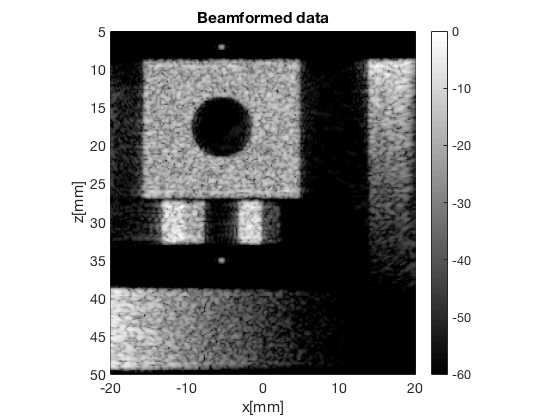
b_data_das.plot();
COHERENCE FACTOR
cf = postprocess.coherence_factor();
cf.dimension = dimension.receive;
cf.receive_apodization = mid.receive_apodization;
cf.transmit_apodization = mid.transmit_apodization;
cf.input = b_data_tx;
b_data_cf = cf.go();
b_data_cf.data = b_data_cf.data.*weights(:); %Compensate for geometrical spreading
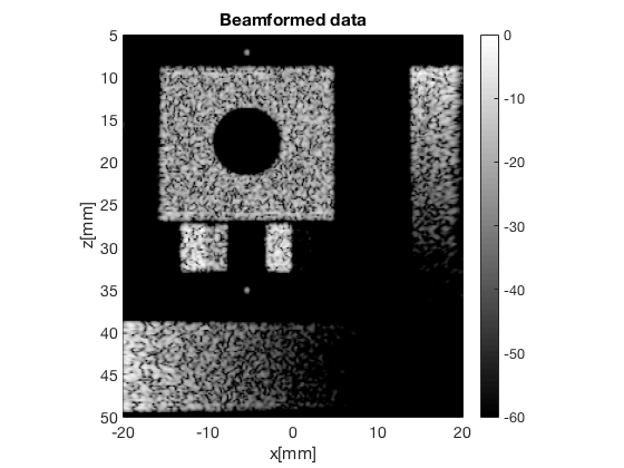
b_data_cf.plot();
uff.apodization: Inputs and outputs are unchanged. Skipping process.
MINIMUM VARIANCE
mv = postprocess.capon_minimum_variance();
mv.dimension = dimension.receive;
mv.transmit_apodization = mid.transmit_apodization;
mv.receive_apodization = mid.receive_apodization;
mv.input = b_data_tx;
mv.scan = scan;
mv.channel_data = channel_data;
mv.K_in_lambda = 1.5;
mv.L_elements = channel_data.probe.N/2;
mv.regCoef = 1/100;
b_data_mv = mv.go();
b_data_mv.data = b_data_mv.data.*weights(:); %Compensate for geometrical spreading
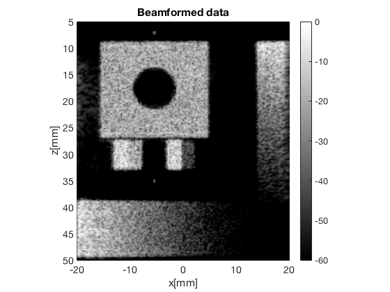
b_data_mv.plot();
uff.apodization: Inputs and outputs are unchanged. Skipping process.
Running the Dynamic Range Test
To run the dynamic range test we call the implementation under tools and pass the channel data object, the beamformed data object an the name of the beamformer.
drt_value_das = tools.dynamic_range_test(channel_data,b_data_das,'DAS')
drt_value_cf = tools.dynamic_range_test(channel_data,b_data_cf,'CF')
drt_value_mv = tools.dynamic_range_test(channel_data,b_data_mv,'MV')
drt_value_das =

  1×2 single row vector

    1.0126    0.9595


drt_value_cf =

  1×2 single row vector

    1.6499    1.4194


drt_value_mv =

  1×2 single row vector

    0.9922    0.9289

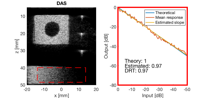
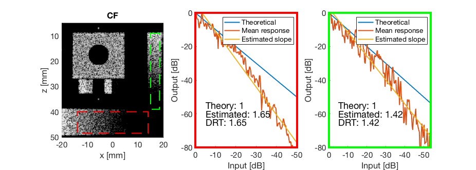
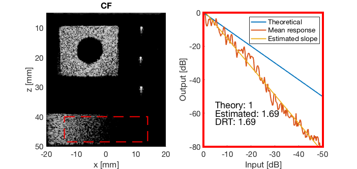
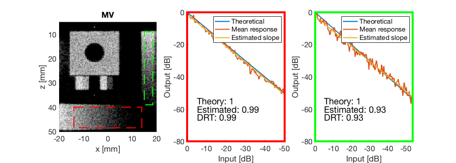
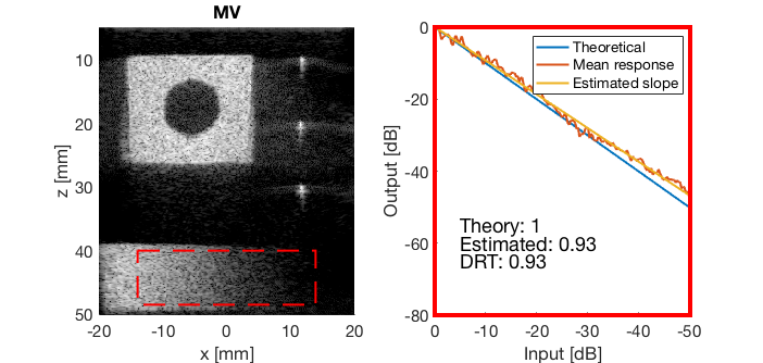
The DRT test reveals that DAS is quite linear for both the simulated and experimental test. The MV compresses the dynamic range slightly, while the CF stretches the dynamic range.