CPWC simulation with the USTB built-in Fresnel simulator

In this example we show how to use the built-in fresnel simulator in USTB to generate a Coherent Plane-Wave Compounding (CPWC) dataset and how it can be beamformed with USTB.

Related materials:

Montaldo et al. 2009

by Alfonso Rodriguez-Molares alfonso.r.molares@ntnu.no 31.03.2017

Phantom
Probe
Pulse
Sequence generation
The Fresnel simulator
Scan
Beamformer

Phantom

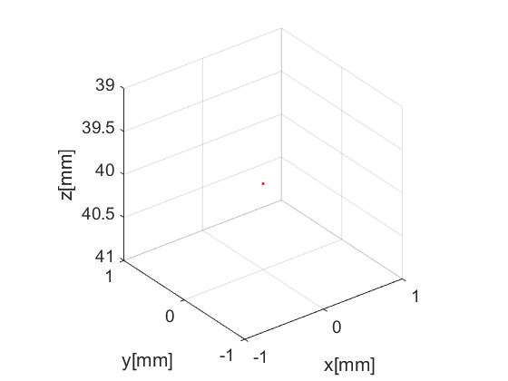
The fresnel simulator takes a phantom structure as input. phantom is an Ultrasound File Format (UFF) structure that contains the position of a collection of point scatterers. USTB's implementation of phantom includes a plot method

pha=uff.phantom();
pha.sound_speed=1540;            % speed of sound [m/s]
pha.points=[0,  0, 40e-3, 1];    % point scatterer position [m]
fig_handle=pha.plot();

Probe

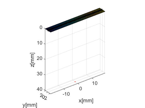
Another UFF structure is probe. You've guessed it, it contains information about the probe's geometry. USTB's implementation comes with a plot method. When combined with the previous Figure we can see the position of the probe respect to the phantom.

prb=uff.linear_array();
prb.N=128;                  % number of elements
prb.pitch=300e-6;           % probe pitch in azimuth [m]
prb.element_width=270e-6;   % element width [m]
prb.element_height=5000e-6; % element height [m]
prb.plot(fig_handle);

Pulse

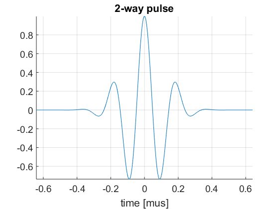
We need to define the pulse-echo signal which is a combination of the electrical pulse sent to each element and the element's electromechanical transfer function. The model used in the built-in fresnel simulator is very simple and it neglects the effect of the spatial impulse response. For a more accurate model, use Field II (http://field-ii.dk/).

In order to define the pulse-echo signal in the fresnel simulator the structure pulse is used:

pul=uff.pulse();
pul.center_frequency=5.2e6;       % transducer frequency [MHz]
pul.fractional_bandwidth=0.6;     % fractional bandwidth [unitless]
pul.plot([],'2-way pulse');

Sequence generation

Here comes something a bit more interesting. The fresnel simulator takes the same sequence definition as the USTB beamformer. In UFF and USTB a sequence is defined as a collection of wave.

The most important piece of information in a wave structure is the the location of the source that generated the wavefront. For the case of a plane-wave with inclination $\alpha$ the source is placed at the location $(r,\theta,\phi)=(\infty,\alpha,0)$ .

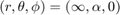For flexibility reasons the wave structure holds all the information needed to beamform that specific transmitted wave, i.e. probe dimensions and reference sound speed. That adds some data overhead, since the probe and sound speed are often the same for all transmit events in the sequence. But it makes it possible to process each transmitting event independently. On the other hand it also simplifies the handling of probes with multiplexors and even allows for a more efficient use of the memory in those cases.

We define a sequence of 31 plane-waves covering an angle span of $[-0.3, 0.3]$ radians. The wave structure has a plot method which plots the direction of the transmitted plane-wave.

N=31;                           % number of plane waves
angles=linspace(-0.3,0.3,N);    % angle vector [rad]
seq=uff.wave();
for n=1:N
    seq(n)=uff.wave();

    seq(n).source.azimuth=angles(n);
    seq(n).source.distance=Inf;

    seq(n).probe=prb;

    seq(n).sound_speed=pha.sound_speed;

    % show source
    fig_handle=seq(n).source.plot(fig_handle);
end

The Fresnel simulator

We can finally launch the built-in simulator. This simulator uses fresnel approximation for a directive rectangular element. We need to assign the phantom, pulse, probe, sequence of wave, and the desired sampling frequency. The simulator returns a channel_data UFF structure.

sim=fresnel();

% setting input data
sim.phantom=pha;                % phantom
sim.pulse=pul;                  % transmitted pulse
sim.probe=prb;                  % probe
sim.sequence=seq;               % beam sequence
sim.sampling_frequency=41.6e6;  % sampling frequency [Hz]

% we launch the simulation
channel_data=sim.go();

USTB's Fresnel impulse response simulator (v1.0.5)
---------------------------------------------------------------

Scan

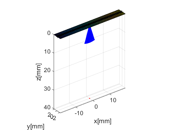
The scan area is defined as a collection of pixels via another UFF structure. The scan is a general structure where the pixels have no spatial organization. That makes it very flexible, but a bit cumbersome to work with. But scan class has a number of children to help with that. In particular we here use the linear_scan structure, which is defined with just two axes. The plot method shows the position of the pixels in a 3D scenario.

sca=uff.linear_scan(linspace(-3e-3,3e-3,200).', linspace(39e-3,43e-3,200).');
sca.plot(fig_handle,'Scenario');    % show mesh

Beamformer

With channel_data and a scan we have all we need to produce an ultrasound image. We now use a USTB structure beamformer, that takes an apodization structure in addition to the channel_data and scan.

bmf=beamformer();
bmf.channel_data=channel_data;
bmf.scan=sca;

bmf.receive_apodization.window=uff.window.tukey50;
bmf.receive_apodization.f_number=1.7;
bmf.receive_apodization.apex.distance=Inf;

bmf.transmit_apodization.window=uff.window.tukey50;
bmf.transmit_apodization.f_number=1.7;
bmf.transmit_apodization.apex.distance=Inf;

The beamformer structure allows you to implement different beamformers by combination of multiple built-in processes. The aim is to avoid code repetition and minimize implementation differences that could hinder inter-comparison. Here we combine two processes (das_matlab and coherent_compounding) to produce coherently compounded images with a MATLAB implementation of the DAS general beamformer.

By changing the process chain other beamforming sequences can be implemented. For instance, in conventional focus imaging each transmit wave leads to a single scan line. In the end all the scanlines are stacked to produce a 2D image. In CPWC, however, a full image is produced for each transmit wave, the so called "low resolution image". Then all the images are coherently combined, i.e. added together, to produce a "high resolution image". Notice that the exact same process is used in other sequences such as DWI or RTB.

This division of the beamforming processing in processes is slower than combining the stages together in a single code, but it opens endless posibilities for implementing different techniques based on the same code blocks.

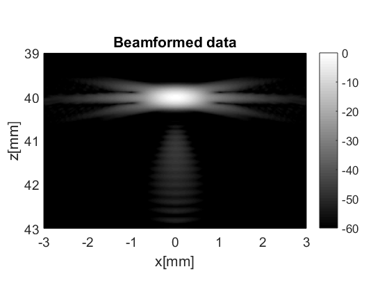
The beamformer returns yet another UFF structure: beamformed_data which we can just display by using the method plot

% beamforming
b_data=bmf.go({process.das_matlab() process.coherent_compounding()});

% show
b_data.plot();