CPWC Fresnel simulation beamformed with the Coherence Factor process

In this example we show how to use the built-in fresnel simulator in USTB to generate a Coherent Plane-Wave Compounding (CPWC) dataset. We then demonstrate how you can use the coherence factor process to do the USTB beamforming with the "adaptive" coherence factor beamforming.

Related materials:

_by Alfonso Rodriguez-Molares alfonso.r.molares@ntnu.no 05.05.2017 and Ole Marius Hoel Rindal olemarius@olemarius.net _

Contents

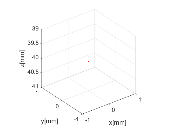
Phantom

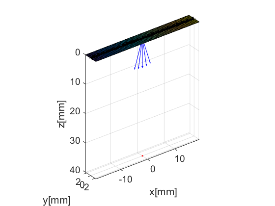
The fresnel simulator takes a phantom structure as input. phantom is an Ultrasound File Format (UFF) structure that contains the position of a collection of point scatterers. USTB's implementation of phantom includes a plot method

pha=uff.phantom();
pha.sound_speed=1540;            % speed of sound [m/s]
pha.points=[0,  0, 40e-3, 1];    % point scatterer position [m]
fig_handle=pha.plot();

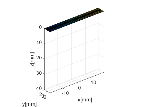
Probe

Another UFF structure is probe. You've guessed it, it contains information about the probe's geometry. USTB's implementation comes with a plot method. When combined with the previous Figure we can see the position of the probe respect to the phantom.

prb=uff.linear_array();
prb.N=128;                  % number of elements
prb.pitch=300e-6;           % probe pitch in azimuth [m]
prb.element_width=270e-6;   % element width [m]
prb.element_height=5000e-6; % element height [m]
prb.plot(fig_handle);

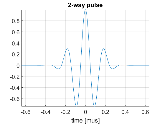
Pulse

We need to define the pulse-echo signal which is a combination of the electrical pulse sent to each element and the element's electromechanical transfer function. The model used in the built-in fresnel simulator is very simple and it neglects the effect of the spatial impulse response. For a more accurate model, use Field II (http://field-ii.dk/).

In order to define the pulse-echo signal in the fresnel simulator the structure pulse is used:

pul=uff.pulse();
pul.center_frequency=5.2e6;       % transducer frequency [MHz]
pul.fractional_bandwidth=0.6;     % fractional bandwidth [unitless]
pul.plot([],'2-way pulse');

Sequence generation

Here comes something a bit more interesting. The fresnel simulator takes the same sequence definition as the USTB beamformer. In UFF and USTB a sequence is defined as a collection of wave.

The most important piece of information in a wave structure is the the location of the source that generated the wavefront. For the case of a plane-wave with inclination the source is placed at the location .

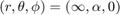For flexibility reasons the wave structure holds all the information needed to beamform that specific transmitted wave, i.e. probe dimensions and reference sound speed. That adds some data overhead, since the probe and sound speed are often the same for all transmit events in the sequence. But it makes it possible to process each transmitting event independently. On the other hand it also simplifies the handling of probes with multiplexors and even allows for a more efficient use of the memory in those cases.

We define a sequence of 31 plane-waves covering an angle span of radians. The wave structure has a plot method which plots the direction of the transmitted plane-wave.

N=5;                           % number of plane waves
angles=linspace(-0.3,0.3,N);    % angle vector [rad]
seq=uff.wave();
for n=1:N
    seq(n)=uff.wave();

    seq(n).source.azimuth=angles(n);
    seq(n).source.distance=Inf;

    seq(n).probe=prb;

    seq(n).sound_speed=pha.sound_speed;

    % show source
    fig_handle=seq(n).source.plot(fig_handle);
end

The Fresnel simulator

We can finally launch the built-in simulator. This simulator uses fresnel approximation for a directive rectangular element. We need to assign the phantom, pulse, probe, sequence of wave, and the desired sampling frequency. The simulator returns a channel_data UFF structure.

sim=fresnel();

% setting input data
sim.phantom=pha;                % phantom
sim.pulse=pul;                  % transmitted pulse
sim.probe=prb;                  % probe
sim.sequence=seq;               % beam sequence
sim.sampling_frequency=41.6e6;  % sampling frequency [Hz]

% we launch the simulation
channel_data=sim.go();

USTB's Fresnel impulse response simulator (v1.0.5)
---------------------------------------------------------------

Scan

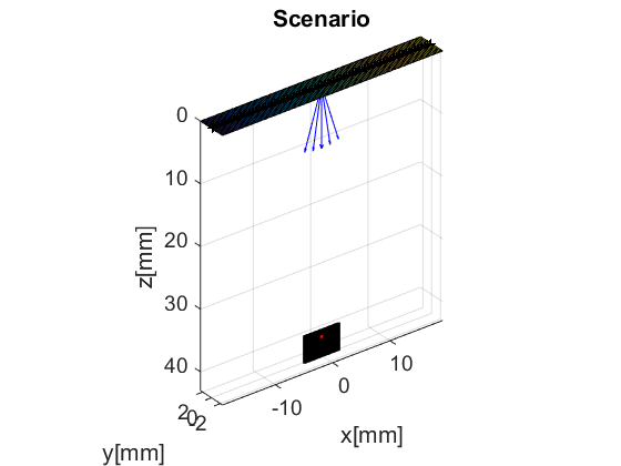
The scan area is defined as a collection of pixels via another UFF structure. The scan is a general structure where the pixels have no spatial organization. That makes it very flexible, but a bit cumbersome to work with. But scan class has a number of children to help with that. In particular we here use the linear_scan structure, which is defined with just two axes. The plot method shows the position of the pixels in a 3D scenario.

sca=uff.linear_scan(linspace(-3e-3,3e-3,200).', linspace(39e-3,43e-3,200).');
sca.plot(fig_handle,'Scenario');    % show mesh

Beamformer

With channel_data and a scan we have all we need to produce an ultrasound image. We now use a USTB structure beamformer, that takes an apodization structure in addition to the channel_data and scan.

bmf=beamformer();
bmf.channel_data=channel_data;
bmf.scan=sca;

bmf.receive_apodization.window=uff.window.boxcar;
bmf.receive_apodization.f_number=1.7;
bmf.receive_apodization.apex.distance=Inf;

%We set this to none since we want to examin the low quality PW images
bmf.transmit_apodization.window=uff.window.none;
bmf.transmit_apodization.f_number=1.7;
bmf.transmit_apodization.apex.distance=Inf;

delay beamforming

b_data = bmf.go({process.delay_matlab()});

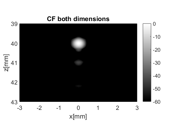
CF on both transmit and receive

proc_cf=process.coherence_factor();
proc_cf.beamformed_data=b_data;
proc_cf.channel_data=bmf.channel_data;
proc_cf.transmit_apodization=bmf.transmit_apodization;
proc_cf.receive_apodization=bmf.receive_apodization;
bmf_data_cf = proc_cf.go();
bmf_data_cf.plot([],'CF both dimensions')

ans = 

  Figure (9) with properties:

      Number: 9
        Name: ''
       Color: [0.9400 0.9400 0.9400]
    Position: [680 558 560 420]
       Units: 'pixels'

  Use GET to show all properties

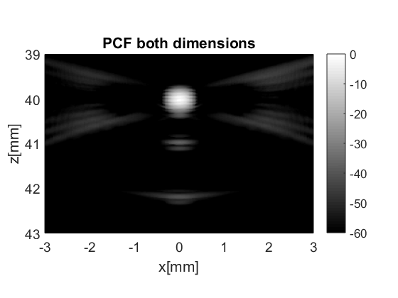
PCF on both transmit and receive

proc_pcf=process.phase_coherence_factor_alternative();
proc_pcf.beamformed_data=b_data;
proc_pcf.channel_data=bmf.channel_data;
proc_pcf.transmit_apodization=bmf.transmit_apodization;
proc_pcf.receive_apodization=bmf.receive_apodization;
bmf_data_pcf = proc_pcf.go();
bmf_data_pcf.plot([],'PCF both dimensions')

ans = 

  Figure (12) with properties:

      Number: 12
        Name: ''
       Color: [0.9400 0.9400 0.9400]
    Position: [680 558 560 420]
       Units: 'pixels'

  Use GET to show all properties

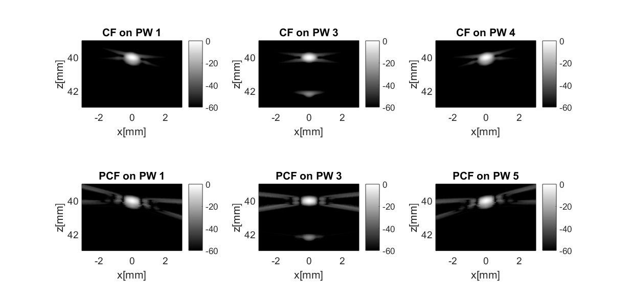
CF "receive" dimension resulting in individual CF PW images

rx_cf=process.coherence_factor();
rx_cf.beamformed_data=b_data;
rx_cf.channel_data=bmf.channel_data;
rx_cf.transmit_apodization=bmf.transmit_apodization;
rx_cf.receive_apodization=bmf.receive_apodization;
rx_cf.dimension=dimension.receive;
bmf_data_rx_cf=rx_cf.go();

PCF "receive" dimension resulting in individual CF PW images

rx_pcf=process.phase_coherence_factor_alternative();
rx_pcf.beamformed_data=b_data;
rx_pcf.channel_data=bmf.channel_data;
rx_pcf.transmit_apodization=bmf.transmit_apodization;
rx_pcf.receive_apodization=bmf.receive_apodization;
rx_pcf.dimension=dimension.receive;
bmf_data_rx_pcf=rx_pcf.go();

figure();
ax = subplot(2,3,1);
bmf_data_rx_cf(1,1).plot(ax,['CF on PW 1']);
ax = subplot(2,3,2);
bmf_data_rx_cf(1,round(end/2)).plot(ax,['CF on PW 3']);
ax = subplot(2,3,3);
bmf_data_rx_cf(1,end).plot(ax,['CF on PW 4']);
ax = subplot(2,3,4);
bmf_data_rx_pcf(1,1).plot(ax,['PCF on PW 1']);
ax = subplot(2,3,5);
bmf_data_rx_pcf(1,round(end/2)).plot(ax,['PCF on PW 3']);
ax = subplot(2,3,6);
bmf_data_rx_pcf(1,end).plot(ax,['PCF on PW 5']);
set(gcf,'Position',[ 50 50 1232 592]);

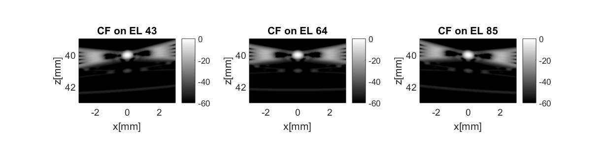
"transmit" dimension CF

proc_cf=process.coherence_factor();
proc_cf.beamformed_data=b_data;
proc_cf.channel_data=bmf.channel_data;
proc_cf.transmit_apodization=bmf.transmit_apodization;
proc_cf.receive_apodization=bmf.receive_apodization;
proc_cf.dimension=dimension.transmit;
cf_data_tx=proc_cf.go();

figure();
ax = subplot(1,3,1);
cf_data_tx(1,43).plot(ax,['CF on EL 43']);
ax = subplot(1,3,2);
cf_data_tx(1,64).plot(ax,['CF on EL 64']);
ax = subplot(1,3,3);
cf_data_tx(1,85).plot(ax,['CF on EL 85']);
set(gcf,'Position',[ 50 150 1232 300]);

"transmit" dimension PCF

fon: this takes too long to be included in the example. Need to review this.

proc_pcf=process.phase_coherence_factor_alternative(); proc_pcf.beamformed_data=b_data; proc_pcf.channel_data=bmf.channel_data; proc_pcf.transmit_apodization=bmf.transmit_apodization; proc_pcf.receive_apodization=bmf.receive_apodization; proc_pcf.dimension=dimension.transmit; pcf_data_tx=proc_pcf.go();

figure(); ax = subplot(1,3,1); pcf_data_tx(1,43).plot(ax,['PCF on EL 43']); ax = subplot(1,3,2); pcf_data_tx(1,64).plot(ax,['PCF on EL 64']); ax = subplot(1,3,3); pcf_data_tx(1,85).plot(ax,['PCF on EL 85']); set(gcf,'Position',[ 50 150 1232 300]);

Published with MATLAB® R2015a