CPWC_linear_array

CPWC movement simulation with the USTB built-in Fresnel simulator
Phantom
Probe
Pulse
Sequence generation
Simulator
Scan
Beamformer

CPWC movement simulation with the USTB built-in Fresnel simulator

In this example we show how to use the built-in fresnel simulator in USTB to generate a Coherent Plane-Wave Compounding (CPWC) squence on a linear array and simulate movement.

Related materials:

Montaldo et al. 2009

by Alfonso Rodriguez-Molares alfonso.r.molares@ntnu.no 13.03.2017 and Arun Asokan nair anair8@jhu.edu

clear all;
close all;

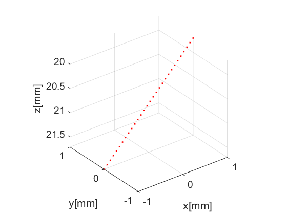
Phantom

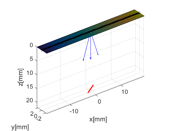
Our first step is to define an appropriate phantom structure as input, or as in this case a series of phantom structures each corresponding to the distribution of point scatterers at a certain point in time. This distribution is determined by the variables defined below.

alpha=-45*pi/180;                 % velocity direction [rad]
N_sca=1;                          % number of scatterers
% x_sca=random('unif',-10e-3,10e-3,N_sca,1); % Uncomment this if using
                                            % multiple scatterers
% z_sca=random('unif',15e-3,25e-3,N_sca,1);  % Uncomment this if using
                                            % multiple scatterers
x_sca=-1e-3;                      % Comment this out if using multiple scatterers
z_sca=21e-3;                      % Comment this out if using multiple scatterers
p=[x_sca zeros(N_sca,1) z_sca+x_sca*sin(alpha)];
v=0.9754*ones(N_sca,1)*[cos(alpha) 0 sin(alpha)]; % scatterer velocity [m/s m/s m/s]
PRF=10000;                           % pulse repetition frequency [Hz]
N_plane_waves=3;                     % number of plane wave
N_frames=10;                         % number of frames
fig_handle=figure();
for n=1:N_plane_waves*N_frames
    pha(n)=uff.phantom();
    pha(n).sound_speed=1540;            % speed of sound [m/s]
    pha(n).points=[p+v*(n-1)/PRF, ones(N_sca,1)];    % point scatterer position [m]
    pha(n).plot(fig_handle);
end

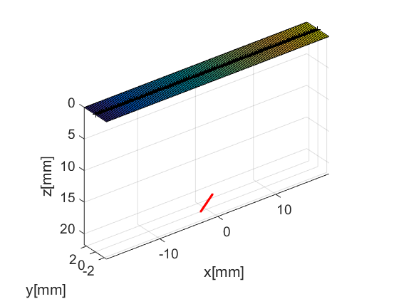
Probe

The next step is to define the probe structure which contains information about the probe's geometry. This too comes with % a plot method that enables visualization of the probe with respect to the phantom. The probe we will use in our example is a linear array transducer with 128 elements.

prb=uff.linear_array();
prb.N=128;                  % number of elements
prb.pitch=300e-6;           % probe pitch in azimuth [m]
prb.element_width=270e-6;   % element width [m]
prb.element_height=5000e-6; % element height [m]
prb.plot(fig_handle);

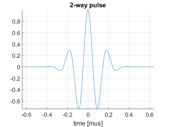
Pulse

We then define the pulse-echo signal which is done here using the fresnel simulator's pulse structure. We could also use 'Field II' for a more accurate model.

pul=uff.pulse();
pul.center_frequency=5.2e6;       % transducer frequency [MHz]
pul.fractional_bandwidth=0.6;     % fractional bandwidth [unitless]
pul.plot([],'2-way pulse');

Sequence generation

Now, we shall generate our sequence! Keep in mind that the fresnel simulator takes the same sequence definition as the USTB beamformer. In UFF and USTB a sequence is defined as a collection of wave structures.

For our example here, we define a sequence of 15 plane-waves covering an angle span of $[-0.3, 0.3]$ radians. The wave structure has a plot method which plots the direction of the transmitted plane-wave.

angles=linspace(-0.3,0.3,N_plane_waves);
seq=uff.wave();
for n=1:N_plane_waves
    seq(n)=uff.wave();

    seq(n).source.azimuth=angles(n);
    seq(n).source.distance=Inf;

    seq(n).probe=prb;

    seq(n).sound_speed=pha.sound_speed;

    % show source
    fig_handle=seq(n).source.plot(fig_handle);
end

Simulator

Finally, we launch the built-in fresnel simulator. The simulator takes in a phantom, pulse, probe and a sequence of wave structures along with the desired sampling frequency, and returns a channel_data UFF structure.

sim=fresnel();

% setting input data
sim.phantom=pha;                % phantom
sim.pulse=pul;                  % transmitted pulse
sim.probe=prb;                  % probe
sim.sequence=seq;               % beam sequence
sim.PRF=PRF;                    % pulse repetition frequency [Hz]
sim.sampling_frequency=41.6e6;  % sampling frequency [Hz]

% we launch the simulation
channel_data=sim.go();

USTB's Fresnel impulse response simulator (v1.0.5)
---------------------------------------------------------------

Scan

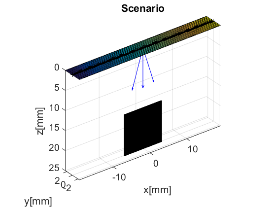
The scan area is defines as a collection of pixels spanning our region of interest. For our example here, we use the linear_scan structure, which is defined with just two axes. scan too has a useful plot method it can call.

sca=uff.linear_scan(linspace(-5e-3,5e-3,256).', linspace(15e-3,25e-3,256).');
sca.plot(fig_handle,'Scenario');    % show mesh

Beamformer

With channel_data and a scan we have all we need to produce an ultrasound image. We now use a USTB structure beamformer, that takes an apodization structure in addition to the channel_data and scan.

bmf=beamformer();
bmf.channel_data=channel_data;
bmf.scan=sca;

bmf.receive_apodization.window=uff.window.tukey50;
bmf.receive_apodization.f_number=1.0;
bmf.receive_apodization.apex.distance=Inf;

bmf.transmit_apodization.window=uff.window.tukey50;
bmf.transmit_apodization.f_number=1.0;
bmf.transmit_apodization.apex.distance=Inf;

Go beamformer! % The beamformer structure allows you to implement different beamformers by combination of multiple built-in processes. Here, we shall use delay-and-sum (implemented in MATLAB); there is a MEX implementation too that we could call with process.das_mex(). In addition, we shall chain it with the process.coherent_compounding() to coherently compound the individual plane wave images.

b_data=bmf.go({process.das_matlab() process.coherent_compounding()});

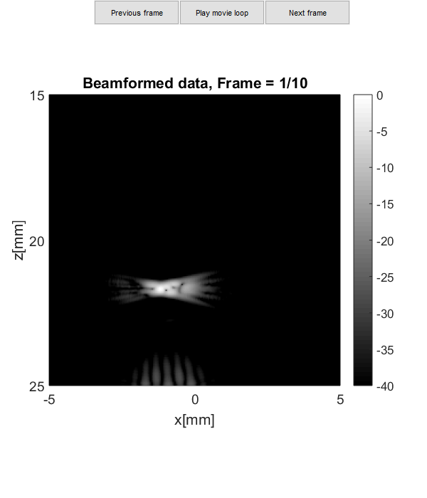
Finally, show our results

b_data.plot([],['Beamformed data'],40);

Contents