Contents
- Multiple line aqusition (MLA) and retrospective beamformgin (RTB) for a phased array sector scan
- Create the sector scan we want to reconstruct
- Conventional Scanline Beamforming
- Define scan with 8 MLA's
- MLA beamforming with conventional virtual source model
- MLA beamforming with Nguyen & Prager model
- MLA beamforming using our simple model assuming PW around focus
- Lets have a closer look at the focal region
- RTB using convetional virtual source model
- Get the transmit apod to give the image correct weighting
- RTB with Nguyen & Prager model
- RTB with hybrid PW model
Multiple line aqusition (MLA) and retrospective beamformgin (RTB) for a phased array sector scan
This script is available in the USTB repository as examples/uff/FI_UFF_phased_array_MLA_and_RTB_fix.m
This example demonstrates the MLA and RTB implementation and demonstrates different fixes to the artifact occuring near the focus for a sector scan.
One solution is the transmit delay model introduced in Nguyen, N. Q., & Prager, R. W. (2016). High-Resolution Ultrasound Imaging With Unified Pixel-Based Beamforming. IEEE Trans. Med. Imaging, 35(1), 98-108.
Another solution is a simpler model assuming PW around focus.
_by Ole Marius Hoel Rindal olemarius@olemarius.net Last updated: 2018/10/05
% Clear up
clear all; close all;

% Read the data, poentitally download it
url='http://ustb.no/datasets/';      % if not found downloaded from here
local_path = [ustb_path(),'/data/']; % location of example data
addpath(local_path);

% Choose dataset
filename='P4_FI.uff';

% check if the file is available in the local path or downloads otherwise
tools.download(filename, url, local_path);
channel_data = uff.read_object([local_path, filename],'/channel_data');
UFF: reading channel_data [uff.channel_data]
UFF: reading sequence [uff.wave] [====================] 100%
Create the sector scan we want to reconstruct
scan=uff.sector_scan('azimuth_axis',...
    linspace(channel_data.sequence(1).source.azimuth,...
                channel_data.sequence(end).source.azimuth,...
                length(channel_data.sequence))',...
    'depth_axis',linspace(0,90e-3,512)');
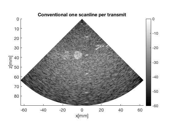
Conventional Scanline Beamforming
mid = midprocess.das();
mid.channel_data=channel_data;
mid.dimension = dimension.both();
mid.scan=scan;
mid.transmit_apodization.window=uff.window.scanline;
mid.receive_apodization.window=uff.window.tukey25;
mid.receive_apodization.f_number = 1.7;

b_data = mid.go();
USTB General beamformer MEX v1.1.2 .............done!
Display image
b_data.plot(40,['Conventional one scanline per transmit']);
Define scan with 8 MLA's
MLA = 8;
scan_MLA=uff.sector_scan('azimuth_axis',...
    linspace(scan.azimuth_axis(1),scan.azimuth_axis(end),...
    scan.N_azimuth_axis*MLA)'...
    ,'depth_axis',scan.depth_axis);
MLA beamforming with conventional virtual source model
mid_MLA=midprocess.das();
mid_MLA.channel_data=channel_data;
mid_MLA.dimension = dimension.both();
mid_MLA.scan=scan_MLA;
mid_MLA.transmit_apodization.window=uff.window.scanline;
mid_MLA.transmit_apodization.MLA = MLA;
mid_MLA.transmit_apodization.MLA_overlap = MLA;
mid_MLA.receive_apodization.window=uff.window.tukey25;
mid_MLA.receive_apodization.f_number = 1.7;

b_data_MLA = mid_MLA.go();
USTB General beamformer MEX v1.1.2 .............done!
Plot the image
b_data_MLA.plot(41,['MLA image conventional virtual source model']);

Notice the artifact seen at radial distance about 50 mm from the origin, yes the artifact can be somewhat hard to see. It will be easier to see in the images that are zoomed in.
MLA beamforming with Nguyen & Prager model
mid_MLA_unified_fix=midprocess.das();
mid_MLA_unified_fix.channel_data=channel_data;
mid_MLA_unified_fix.dimension = dimension.both();
%By setting this we use the Prager & Nguyen model
mid_MLA_unified_fix.use_unified_fix = 1;
mid_MLA_unified_fix.scan=scan_MLA;
mid_MLA_unified_fix.transmit_apodization.window=uff.window.scanline;
mid_MLA_unified_fix.transmit_apodization.MLA = MLA;
mid_MLA_unified_fix.transmit_apodization.MLA_overlap = MLA;
mid_MLA_unified_fix.receive_apodization.window=uff.window.tukey25;
mid_MLA_unified_fix.receive_apodization.f_number = 1.7;

b_data_MLA_unified_fix = mid_MLA_unified_fix.go();
USTB General beamformer MEX v1.1.2 .............done!
Plot the image
b_data_MLA_unified_fix.plot(42,['MLA image Nguyen & Prager model']);
ax(4) = gca;
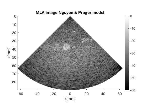
Notice that the artifact is gone
MLA beamforming using our simple model assuming PW around focus
mid_MLA_plane_fix=midprocess.das();
mid_MLA_plane_fix.channel_data=channel_data;
mid_MLA_plane_fix.dimension = dimension.both();
%By setting this we use the simple PW model
mid_MLA_plane_fix.use_PW_fix = 1;
mid_MLA_plane_fix.margin_in_m = 4/1000;
mid_MLA_plane_fix.scan=scan_MLA;
mid_MLA_plane_fix.transmit_apodization.window=uff.window.scanline;
mid_MLA_plane_fix.transmit_apodization.MLA = MLA;
mid_MLA_plane_fix.transmit_apodization.MLA_overlap = MLA;
mid_MLA_plane_fix.receive_apodization.window=uff.window.tukey25;
mid_MLA_plane_fix.receive_apodization.f_number = 1.7;

b_data_MLA_plane_fix = mid_MLA_plane_fix.go();
USTB General beamformer MEX v1.1.2 .............done!
Plot the image
b_data_MLA_plane_fix.plot(43,['MLA image with PW hybrid virtual source model']);

Notice that the artifact is gone.
Lets have a closer look at the focal region
Both regions fix the focal region in front of the tranducer
f100 = figure(100);
set(f100,'Position',[260     6   526   694]);
b_data.plot(subplot(4,2,1),['No MLAs']);
ax_sub_top(1) = gca;
b_data_MLA.plot(subplot(4,2,2),['MLAs virtual source']);
ax_sub_top(2) = gca;
b_data_MLA_unified_fix.plot(subplot(4,2,3),['MLAs using Nguyen & Prager']);
ax_sub_top(3) = gca;
b_data_MLA_plane_fix.plot(subplot(4,2,4),['MLAs using PW model']);
ax_sub_top(4) = gca;
linkaxes(ax_sub_top)
ylim([45 60]);xlim([-10 10]);

b_data.plot(subplot(4,2,5),['No MLAs']);
ax_sub_bottom(1) = gca;
b_data_MLA.plot(subplot(4,2,6),['MLAs virtual source']);
ax_sub_bottom(2) = gca;
b_data_MLA_unified_fix.plot(subplot(4,2,7),['MLAs using Nguyen & Prager']);
ax_sub_bottom(3) = gca;
b_data_MLA_plane_fix.plot(subplot(4,2,8),['MLAs using PW model']);
ax_sub_bottom(4) = gca;
linkaxes(ax_sub_bottom)
ylim([40 55]);xlim([15 35]);
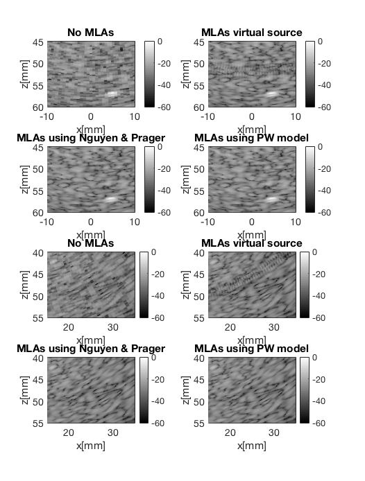
We can observe that the artifact is removed for both the Nguyen & Prager model, and our simple PW model both in front front of the probe (around x=0mm), and to the side (x=25mm) which was an earlier issue.
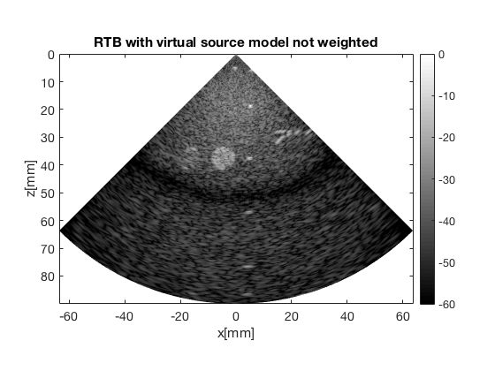
RTB using convetional virtual source model
mid_RTB=midprocess.das();
mid_RTB.channel_data=channel_data;
mid_RTB.dimension = dimension.both();
mid_RTB.scan=scan_MLA;
mid_RTB.transmit_apodization.window = uff.window.sector_scan_rtb;
mid_RTB.transmit_apodization.probe = channel_data.probe;
mid_RTB.receive_apodization.window = uff.window.tukey25;
mid_RTB.receive_apodization.f_number = 1.7;

b_data_RTB = mid_RTB.go();
USTB General beamformer MEX v1.1.2 .............done!
Display image withough weighting
b_data_RTB.plot([],['RTB with virtual source model not weighted']);
Get the transmit apod to give the image correct weighting
tx_apod = mid_RTB.transmit_apodization.data;

x_matrix=reshape(scan_MLA.x,[scan_MLA.N_depth_axis scan_MLA.N_azimuth_axis]);
z_matrix=reshape(scan_MLA.z,[scan_MLA.N_depth_axis scan_MLA.N_azimuth_axis]);

figure(88);
pcolor(x_matrix*1e3,z_matrix*1e3,...
       reshape(tx_apod(:,51),scan_MLA.N_depth_axis,scan_MLA.N_azimuth_axis));
xlabel('x [mm]');
ylabel('z [mm]');
shading('flat');
set(gca,'fontsize',14);
set(gca,'YDir','reverse');
axis('tight','equal');
title('TX apod from sequence 51');
uff.apodization: Inputs and outputs are unchanged. Skipping process.
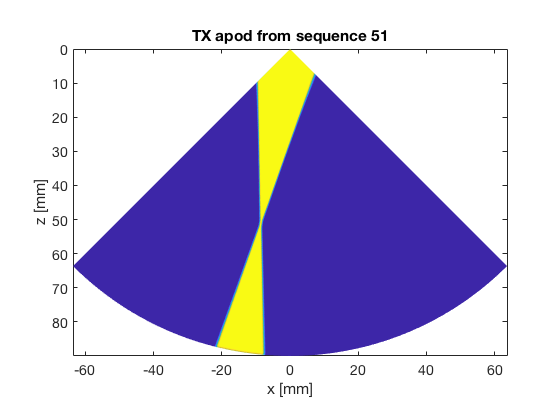
For illustrational purposes, we'll include a plot of the transmit apodization
% Calculate weights based on the transmit apod
weighting = 1./sum(tx_apod,2);

b_data_RTB_weighted = uff.beamformed_data(b_data_RTB);
b_data_RTB_weighted.data = b_data_RTB_weighted.data.*weighting;

b_data_RTB_weighted.plot(11,'RTB with virtual source model weighted');
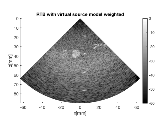
Notice that we once again have the artifact around focus
RTB with Nguyen & Prager model
mid_RTB_unified_fix=midprocess.das();
mid_RTB_unified_fix.channel_data=channel_data;
mid_RTB_unified_fix.dimension = dimension.both();
mid_RTB_unified_fix.use_unified_fix = 1;
mid_RTB_unified_fix.scan=scan_MLA;
mid_RTB_unified_fix.transmit_apodization.window = uff.window.sector_scan_rtb;
mid_RTB_unified_fix.transmit_apodization.probe = channel_data.probe;
mid_RTB_unified_fix.receive_apodization.window = uff.window.tukey25;
mid_RTB_unified_fix.receive_apodization.f_number = 1.7;

b_data_RTB_unified_fix = mid_RTB_unified_fix.go();

b_data_RTB_unified_fix_weighted = uff.beamformed_data(b_data_RTB_unified_fix);
b_data_RTB_unified_fix_weighted.data = b_data_RTB_unified_fix_weighted.data.*weighting;
USTB General beamformer MEX v1.1.2 .............done!
Plot the weighted image
b_data_RTB_unified_fix_weighted.plot(12,'RTB with Nguyen & Prager model');

Notice that the artifact around focus is removed
RTB with hybrid PW model
mid_RTB_PW_fix=midprocess.das();
mid_RTB_PW_fix.channel_data=channel_data;
mid_RTB_PW_fix.dimension = dimension.both();
mid_RTB_PW_fix.use_PW_fix = 1;
mid_RTB_PW_fix.margin_in_m = 4/1000;
mid_RTB_PW_fix.scan=scan_MLA;
mid_RTB_PW_fix.transmit_apodization.window = uff.window.sector_scan_rtb;
mid_RTB_PW_fix.transmit_apodization.probe = channel_data.probe;
mid_RTB_PW_fix.receive_apodization.window = uff.window.tukey25;
mid_RTB_PW_fix.receive_apodization.f_number = 1.7;

b_data_RTB_PW_fix = mid_RTB_PW_fix.go();

b_data_RTB_PW_fix_weighted = uff.beamformed_data(b_data_RTB_PW_fix);
b_data_RTB_PW_fix_weighted.data = b_data_RTB_PW_fix_weighted.data.*weighting;

b_data_RTB_PW_fix_weighted.plot(13,'RTB with hybrid PW model');
USTB General beamformer MEX v1.1.2 .............done!
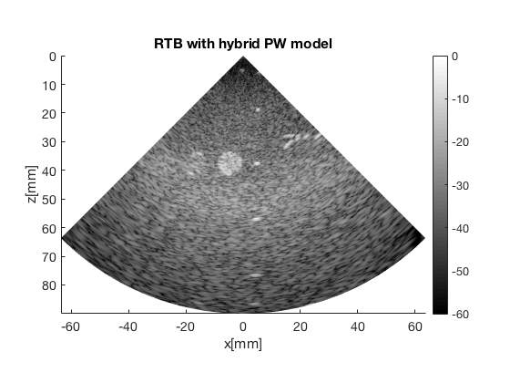
Notice that the artifact around focus is removed
f200 = figure(200);
set(f200,'Position',[260     6   526   694]);
b_data.plot(subplot(4,2,1),['No RTB']);
ax_sub_top(1) = gca;
b_data_RTB_weighted.plot(subplot(4,2,2),['RTB virtual source']);
ax_sub_top(2) = gca;
b_data_RTB_unified_fix_weighted.plot(subplot(4,2,3),['RTB using Nguyen & Prager']);
ax_sub_top(3) = gca;
b_data_RTB_PW_fix_weighted.plot(subplot(4,2,4),['RTB using PW model']);
ax_sub_top(4) = gca;
linkaxes(ax_sub_top)
ylim([45 60]);xlim([-10 10]);

b_data.plot(subplot(4,2,5),['No RTB']);
ax_sub_bottom(1) = gca;
b_data_RTB_weighted.plot(subplot(4,2,6),['RTB virtual source']);
ax_sub_bottom(2) = gca;
b_data_RTB_unified_fix_weighted.plot(subplot(4,2,7),['RTB using Nguyen & Prager']);
ax_sub_bottom(3) = gca;
b_data_RTB_PW_fix_weighted.plot(subplot(4,2,8),['RTB using PW model']);
ax_sub_bottom(4) = gca;
linkaxes(ax_sub_bottom)
ylim([40 55]);xlim([15 35]);
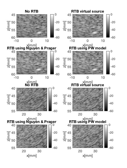
We can observe that the artifact is removed also for RTB beamforming, for both the Nguyen & Prager model, and our simple PW model both in front front of the probe (around x=0mm), and to the side (x=25mm) which was an earlier issue.