Demonstrating the Short Lag Spatial Coherence beamforming algorithm

This example script demonstates the Short Lag Spatial Coherence beamforming algorithm introduced in the article: Lediju, M. A., Trahey, G. E., Byram, B. C., & Dahl, J. J. (2011). Short-lag spatial coherence of backscattered echoes: Imaging characteristics. IEEE Transactions on Ultrasonics, Ferroelectrics, and Frequency Control, 58(7), 1377-1388. https://doi.org/10.1109/TUFFC.2011.1957

The algorithm is demonstrated on a dataset recorded from a standard CIRS phantom of string targets and a hyperechoic cyst. Also, the second part of the example uses a dataset recorded from the parasternal long axis of a human heart. The cardiac SLSC image reproduces the results in the article: Lediju Bell, M. A., Goswami, R., Kisslo, J. A., Dahl, J. J., & Trahey, G. E. (2013). Short-Lag Spatial Coherence (SLSC) Imaging of Cardiac Ultrasound Data: Initial Clinical Results. Ultrasound in Medicine & Biology, 39(10), 1861-1874. https://doi.org/10.1016/j.ultrasmedbio.2013.03.029 However, those results were from parasternal short axis and apical four chamber views, while we show images of the parasternal long axis.

by Ole Marius Hoel Rindal olemarius@olemarius.net and Muyinatu Lediju Bell mledijubell@jhu.edu 21.08.2017

Contents

Reading the UFF dataset

We'll start with reading the UFF dataset recorded from a CIRS phantom

clear all; close all;

% data location
url='http://ustb.no/datasets/';      % if not found download from here
local_path = [ustb_path(),'/data/']; % location of example data
addpath(local_path);

% Choose dataset
filename='Alpinion_L3-8_FI_hyperechoic_scatterers.uff';
% check if the file is available in the local path or downloads otherwise
tools.download(filename, url, local_path);
channel_data = uff.read_object([local_path, filename],'/channel_data');
channel_data.print_authorship

UFF: reading channel_data [uff.channel_data]
UFF: reading sequence [uff.wave] [====================] 100%
Name: 		 FI dataset of hyperechoic cyst and points  
		 scatterers recorded on an Alpinion scanner with a  
		 L3-8 Probe from a CIRS General Purpose Ultrasound  
		 Phantom 
Reference: 	 www.ultrasoundtoolbox.com 
Author(s): 	 Ole Marius Hoel Rindal <olemarius@olemarius.net> 
		 Muyinatu Lediju Bell <mledijubell@jhu.edu> 
Version: 	 1.0.2 

Defining scan for the FI (Focused Imaging) CIRS dataset

Define the scan from z = 0 to 55 mm, the x is defined from the transmit sequence origin position for each scan line.

z_axis=linspace(0e-3,55e-3,512).';
scan=uff.linear_scan();
idx = 1;
for n=1:numel(channel_data.sequence)
    scan(n)=uff.linear_scan();
    scan(n).x_axis = channel_data.sequence(n).source.x;
    scan(n).z_axis = z_axis;
end

Delay the channel data

We are using no apodization because the SLSC algorithm requires equally weighted channel data from all receive elements

bmf=beamformer();
bmf.channel_data=channel_data;
bmf.scan=scan;
bmf.receive_apodization.window=uff.window.none;
b_data=bmf.go({process.delay_mex process.stack});

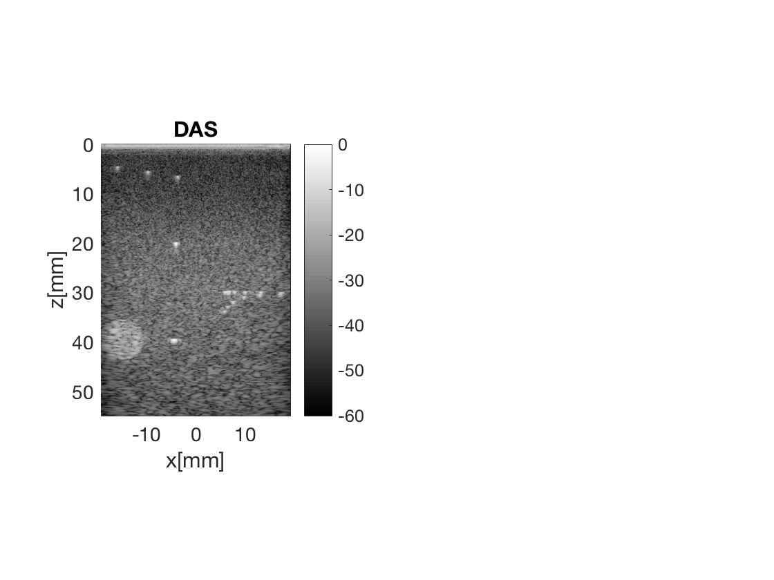
Create the Delay-And-Sum image

das = process.coherent_compounding();
das.beamformed_data = b_data;
das_image = das.go();
figure(1);
das_image.plot(subplot(121),['DAS'],60,'log');

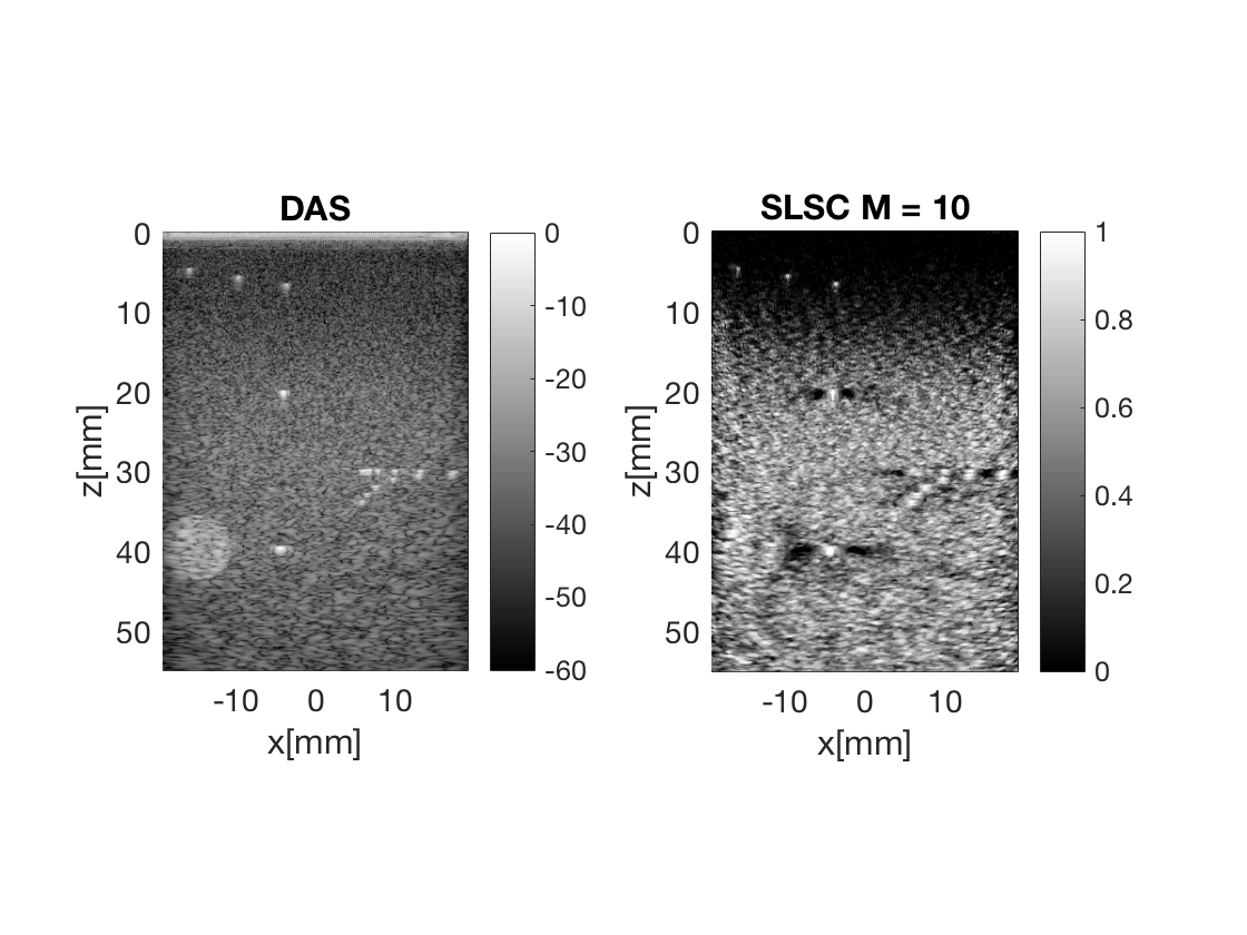
Create the Short Lag Spatial Coherence (SLSC) image

We are using a kernel size equal to one wavelength, and use M = 10. See the article referenced for more details.

slsc = process.short_lag_spatial_coherence();
slsc.receive_apodization = bmf.receive_apodization;
slsc.dimension = dimension.receive;
slsc.channel_data = bmf.channel_data;
slsc.scan = bmf.scan;
slsc.maxM = 10;
slsc.K_in_lambda = 1;
slsc.beamformed_data = b_data;
slsc_data = slsc.go();

The reference of the SLSC process

Let's look at the reference for the SLSC process. If you use the USTB and are using the SLSC process in your work you have to reference this reference according to our citation policy, see http://www.ustb.no/citation/

slsc.print_reference

Reference:	 Lediju, M. A., Trahey, G. E., Byram, B. C., & Dahl 
		 , J. J. (2011). Short-lag spatial coherence of bac 
		 kscattered echoes: Imaging characteristics. IEEE T 
		 ransactions on Ultrasonics, Ferroelectrics, and Fr 
		 equency Control, 58(7), 1377?1388. https://doi.org 
		 /10.1109/TUFFC.2011.1957Lediju Bell, M. A., Goswam 
		 i, R., Kisslo, J. A., Dahl, J. J., & Trahey, G. E. 
		  (2013). Short-Lag Spatial Coherence (SLSC) Imagin 
		 g of Cardiac Ultrasound Data: Initial Clinical Res 
		 ults. Ultrasound in Medicine & Biology, 39(10), 18 
		 61?1874. https://doi.org/10.1016/j.ultrasmedbio.20 
		 13.03.029 

You can also give some credit to the authors of the implementation in your work ;)

slsc.print_implemented_by

Implemented by:	 Ole Marius Hoel Rindal <olemarius@olemarius.net>,  
		 Muyinatu A. Lediju Bell <mledijubell@jhu.edu>, Don 
		 gwoon Hyun <dhyun@stanford.edu> 

Display the SLSC image together with the DAS image

Now, we can finally plot the SLSC image together with the DAS image.

figure(1)
slsc_data.plot(subplot(122),['SLSC M = ',num2str(slsc.maxM)],[],'none');
caxis([0 1])

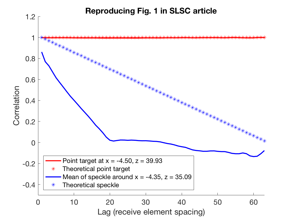
Calculate the full correlation for all 63 lags

The dataset was receving on 64 elements, thus we can calculate the full correlation values for all 63 lags if we want. Then, we can reproduce Fig 1. from Lediju, M. A., Trahey, G. E., Byram, B. C., & Dahl, J. J. (2011). Short-lag spatial coherence of backscattered echoes: Imaging characteristics. IEEE Transactions on Ultrasonics, Ferroelectrics, and Frequency Control, 58(7), 1377?1388. https://doi.org/10.1109/TUFFC.2011.1957

slsc.maxM = 63;
slsc_data = slsc.go();

z_speckle = 327
x_speckle = 100

figure(2);clf;hold all;
plot(squeeze(slsc.slsc_values(372,99,:)),'r','LineWidth',2,'DisplayName',...
    sprintf('Point target at x = %.2f, z = %.2f ',slsc_data.scan.x_axis(99)*1000,...
    slsc_data.scan.z_axis(372)*1000))
plot(ones(1,64),'r*','DisplayName','Theoretical point target')
plot(squeeze(mean(mean(slsc.slsc_values(z_speckle-10:z_speckle+10,x_speckle-10:x_speckle+10,:),2),1)),'b','LineWidth',2,'DisplayName',...
    sprintf('Mean of speckle around x = %.2f, z = %.2f ',slsc_data.scan.x_axis(x_speckle)*1000,...
    slsc_data.scan.z_axis(z_speckle)*1000))
theoretical_speckle = ones(1,64)*64-linspace(1,64,64);
plot(theoretical_speckle./max(theoretical_speckle(:)),'b*','DisplayName','Theoretical speckle')
ylim([-0.5 1.2]); xlim([0 63]);
xlabel('Lag (receive element spacing)'); ylabel('Correlation');
legend('show','Location','sw');
set(gca,'FontSize',14);
title('Reproducing Fig. 1 in SLSC article');

z_speckle =

   327


x_speckle =

   100

SLSC on a cardiac image

Next, let's reproduce some of the results from the article : Lediju Bell, M. A., Goswami, R., Kisslo, J. A., Dahl, J. J., & Trahey, G. E. (2013). Short-Lag Spatial Coherence (SLSC) Imaging of Cardiac Ultrasound Data: Initial Clinical Results. Ultrasound in Medicine & Biology, 39(10), 1861-1874. https://doi.org/10.1016/j.ultrasmedbio.2013.03.029

clear all;close all;
url='http://ustb.no/datasets/';      % if not found downloaded from here
local_path = [ustb_path(),'/data/']; % location of example data
addpath(local_path);
% Choose dataset
filename='Verasonics_P2-4_parasternal_long.uff';
% check if the file is available in the local path or downloads otherwise
tools.download(filename, url, local_path);
channel_data = uff.read_object([local_path, filename],'/channel_data');
scan = uff.read_object([local_path, filename],'/scan');

UFF: reading /channel_data [uff.channel_data]
UFF: reading sequence [uff.wave] [====================] 100%
UFF: reading /scan [uff.sector_scan] [====================] 100%

Print info about the dataset. Remeber that if you want to use this dataset you have to reference this article!

channel_data.print_authorship

Name: 		 A human heart in parasternal long axis, scanned  
		 on the Verasonics 
Reference: 	 Rindal, O. M. H., Aakhus, S., Holm, S., &  
		 Austeng, A. (2017). Hypothesis of Improved  
		 Visualization of Microstructures in the  
		 Interventricular Septum with Ultrasound and  
		 Adaptive Beamforming. Ultrasound in Medicine and  
		 Biology, 43(10), 2494–2499.  
		 https://doi.org/10.1016/j.ultrasmedbio.2017.05.023 
Author(s): 	 Ole Marius Hoel Rindal <olemarius@olemarius.no> 
Version: 	 1.0.0 

Create the images of the heart.

Let's do the same as we did above and create the DAS and the SLSC image of this heart image cycle. Since the code is very similar, we are a bit cheap on the comments ;)

% For the online example we used all the 50 frames in the dataset, but, to
% save time you can scale it down to the number of frames below, if not
% comment the next line out.
% channel_data.N_frames = 5;

bmf=beamformer();
bmf.channel_data=channel_data;
bmf.scan=scan;
bmf.receive_apodization.window=uff.window.none;
% You might notice that I'm using the delay_matlab_light, this is to save
% some precious memory when using all 50 frames :)
b_data=bmf.go({process.delay_matlab_light process.stack});

% DAS image
das = process.coherent_compounding();
das.beamformed_data = b_data;
das_data = das.go();

% SLSC image
slsc = process.short_lag_spatial_coherence();
slsc.receive_apodization = bmf.receive_apodization;
slsc.transmit_apodization = bmf.transmit_apodization;
slsc.dimension = dimension.receive;
slsc.channel_data = bmf.channel_data;
slsc.scan = bmf.scan;
slsc.maxM = 10;
slsc.K_in_lambda = 1;
slsc.beamformed_data = b_data;
slsc_data = slsc.go();

Plot the two images

das_data.plot(3,['DAS']);
slsc_data.plot(4,['SLSC'],[],'none');
caxis([0 1])

Scan Conversion with interpolation

Use the scan conversion from the tools. This is a bit more tricky than the built in, but it adds some interpolation making a final smoother image.

% Get the angles as an array
for tx = 1:numel(channel_data.sequence)
    transmit_angles(tx) = channel_data.sequence(tx).source.azimuth;
end

% Get all the SLSC images as an matrix of images
slsc_images = slsc_data.get_image('none');
das_images = das_data.get_image('log');
%das_images = das_images./max(das_images(:));
% Do the scan conversion for each frame. We are asking for a final image of
% 512x512 samples.
for frame = 1:channel_data.N_frames
    [slsc_interpolated(:,:,frame), Xs, Zs] = tools.scan_convert(slsc_images(:,:,frame),...
        transmit_angles,das_data.scan.depth_axis',512,512);
    [das_interpolated(:,:,frame), Xs, Zs] = tools.scan_convert(das_images(:,:,frame),...
        transmit_angles,das_data.scan.depth_axis',512,512);
end

% Put the data back into uff.beamformed data objects and show them!
slsc_beamformed_img = uff.beamformed_data();
slsc_beamformed_img.scan = uff.linear_scan();
slsc_beamformed_img.scan.x_axis = Xs;
slsc_beamformed_img.scan.z_axis = Zs;
slsc_beamformed_img.data = reshape(slsc_interpolated,...
    size(slsc_interpolated,1)*size(slsc_interpolated,2),size(slsc_interpolated,3));
slsc_beamformed_img.data(slsc_beamformed_img.data==0) = 1; %Make the background white
slsc_beamformed_img.plot(5,'SLSC interpolated',60,'none');
caxis([0 1]);

das_beamformed_img = uff.beamformed_data();
das_beamformed_img.scan = uff.linear_scan();
das_beamformed_img.scan.x_axis = Xs;
das_beamformed_img.scan.z_axis = Zs;
das_beamformed_img.data = reshape(das_interpolated,...
    size(das_interpolated,1)*size(das_interpolated,2),size(das_interpolated,3));
das_beamformed_img.plot(6,'DAS interpolated',60,'none');
caxis([-60 0]);

References

Please see our citation policy http://www.ustb.no/citation/.

If you want to use the SLSC process with the USTB you need to reference this article:

Lediju, M. A., Trahey, G. E., Byram, B. C., & Dahl, J. J. (2011). Short-lag spatial coherence of backscattered echoes: Imaging characteristics. IEEE Transactions on Ultrasonics, Ferroelectrics, and Frequency Control, 58(7), 1377-1388. https://doi.org/10.1109/TUFFC.2011.1957

If you want to use it with cardiac imaging, you also need to reference this article:

Lediju Bell, M. A., Goswami, R., Kisslo, J. A., Dahl, J. J., & Trahey, G. E. (2013). Short-Lag Spatial Coherence (SLSC) Imaging of Cardiac Ultrasound Data: Initial Clinical Results. Ultrasound in Medicine & Biology, 39(10), 1861-1874. https://doi.org/10.1016/j.ultrasmedbio.2013.03.029

If you want to use the dataset from the CIRS phantom, see http://www.ustb.no/ustb-datasets/ and reference the USTB reference.

If you want to use the parasternal long axis cardiac dataset you need to reference this paper. See also http://www.ustb.no/ustb-datasets/:

Rindal, O. M. H., Aakhus, S., Holm, S., & Austeng, A. (2017). Hypothesis of Improved Visualization of Microstructures in the Interventricular Septum with Ultrasound and Adaptive Beamforming. Ultrasound in Medicine and Biology, 43(10), 2494?2499. https://doi.org/10.1016/j.ultrasmedbio.2017.05.023

If you have any questions you can contact the authors of this example.

Published with MATLAB® R2016b