Contents

Achieving uniform field of view (FOV) in synthetic aperture imaging (STAI) in Field II simulations

This exampel investigates and demonstrates how one can achieve uniform field of view in a simulated synthetic aperture imaging ultrasound image from Field II using the correct compensation weighting of the resulting image.

In short, the solution is to make sure you have a uniform pressure field using omnidirectional elements. This is achieved by having both with and height of element smaller than lambda/2. Then one need to have weighting to compensate for the varying array gain from a dynamic aperture (constant f#), and we need weighting to compensate for geometrical spreading.

We'll investiage two cases, the firs is the case of a grid of string targets with uniform intensity, and the second is the case of speckle with uniform intensity in the whole image.

clear all; close all;

Load channel data

The channel data is available from the ustb.no website.

url='http://ustb.no/datasets/';      % if not found downloaded from here
filename = 'FieldII_STAI_uniform_fov.uff';

% Check if the data is allready in your data path, and downloads it otherwise.
% The defaults data path is under USTB's folder, but you can change this
% by setting an environment variable with setenv(DATA_PATH,'the_path_you_want_to_use');
tools.download(filename, url, data_path);

% We'll read two channel data objects. The first is the channel data from asnr_calculated_das_weighted
% grid of strings using a L7-4 probe with element height XX.
channel_data = uff.channel_data();
channel_data.read([data_path filesep filename],'/channel_data');
% The second is the same grid of strings, but with element height lambda/2.
channel_data_lh = uff.channel_data();
channel_data_lh.read([data_path filesep filename],'/channel_data_lh');

UFF: reading channel_data [uff.channel_data]
UFF: reading sequence [uff.wave] [====================] 100%
UFF: reading channel_data_lh [uff.channel_data]
UFF: reading sequence [uff.wave] [====================] 100%

Printing out the different element heights.

channel_data.probe.element_height
channel_data_lh.probe.element_height

ans =

  single

    0.0050


ans =

  single

  1.5000e-04

Define the image scan and beamforming parameters

The scan is defined with x axis equal to the with of the probe, and the z axis goes from 2.5 to 55 mm.

sca=uff.linear_scan('x_axis',linspace(channel_data.probe.x(1),...
    channel_data.probe.x(end),512).','z_axis',linspace(2.5e-3,55e-3,512).');

% We use the Delay-And-Sum beamformer with Tukey 25 windows with f# = 1.7.
% We should, however, obtain the same results and conclusions with other
% windows or a different f#.
mid = midprocess.das();
mid.scan = sca;
mid.channel_data = channel_data;
mid.dimension = dimension.both();
mid.receive_apodization.window=uff.window.tukey25;
mid.receive_apodization.f_number=1.7;
mid.transmit_apodization.window=uff.window.tukey25;
mid.transmit_apodization.f_number=1.7;
b_data = mid.go();

% Interchange the channel data and beamform a second image using the
% dataset simulated with the probe with element height = lambda/2.
mid.channel_data = channel_data_lh;
b_data_lh = mid.go();

USTB General beamformer MEX v1.1.2 .............done!
USTB General beamformer MEX v1.1.2 .............done!

Plot figures of string grid

f1 = figure(1);
set(f1,'Position',[315 106 685 692])
b_data.plot(subplot(2,2,1),'Fig 1: DAS');
b_data_lh.plot(subplot(2,2,3),'Fig 3: DAS elmnt height = \lambda/2');

% To calculate the weights we have to call a tools function called
% *uniform_fov_weighting* with the mid process object as an argument.
[weights,array_gain_compensation,geo_spreading_compensation] = ...
                                           tools.uniform_fov_weighting(mid);

img = b_data.get_image('none');
img_weighted = img.*weights;
img_mod = b_data_lh.get_image('none');
img_mod_weighted = img_mod.*weights;
image.all{1} = db(abs(img./max(img(:))));
image.tags{1} = 'DAS';
image.all{2} = db(abs(img_weighted./max(img_weighted(:))));
image.tags{2} = 'DAS weighted';
image.all{3} = db(abs(img_mod./max(img_mod(:))));
image.tags{3} = 'DAS elmnt height = \lambda/2';
image.all{4} = db(abs(img_mod_weighted./max(img_mod_weighted(:))));
image.tags{4} = 'DAS weighted elmnt height = \lambda/2';

figure(1);
subplot(2,2,2)
imagesc(sca.x_axis*1000,sca.z_axis*1000,image.all{2});
colorbar;
colormap gray; caxis([-60 0]); axis image;
title(['Fig 2: ',image.tags{2}]);xlabel('x[mm]');ylabel('z[mm]')
set(gca,'FontSize',15)
figure(1)
subplot(2,2,4)
imagesc(sca.x_axis*1000,sca.z_axis*1000,image.all{4});
colorbar;
colormap gray; caxis([-60 0]); axis image;
title(['Fig 4: ',image.tags{4}]);xlabel('x[mm]');ylabel('z[mm]')
set(gca,'FontSize',15)

uff.apodization: Inputs and outputs are unchanged. Skipping process.
uff.apodization: Inputs and outputs are unchanged. Skipping process.

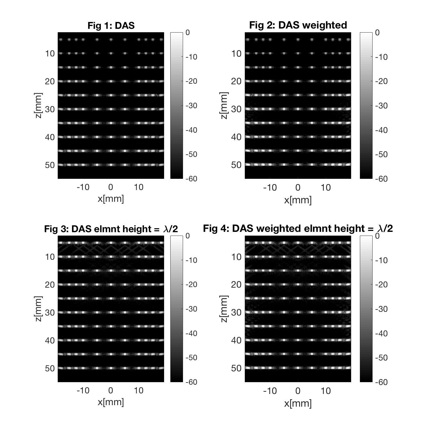
Let's investigate the results. Fig 1 shows the standard DAS image, Fig 2. showns the standard DAS image with the weighting to compensate for the varying array gain from a dynamic aperture (constant f#), and geometrical spreading. Fig 3 is the DAS image from the simulation with omnidirectional elements, height = lambda/2, and Fig 4 is the same image as in Fig 3 but with the compensation weighting. We can observe that the DAS with non-omnidirectional elements in Fig 1 has an intensity varying with depth, but notice that the intensity also drops towards both sides of the image. In Fig 2, the weighting seems to have fixed the problem with the intensity varying towards the sides, but not varying with depth. In Fig 3. we have the DAS image from omnidirectional elements without the weighting. Notice that the intensity varying with depth seems to be fixed by using omnidirectional elements, but the intensity still dropps of towards the sides. Finally, in Fig 4 the DAS image with omnidirectional elements and compensation weigting seems to have an uniform fov.

Investigate weighting compensation

f2 = figure(2);clf;
set(f2,'Position',[142 323 1233 423])
subplot(1,3,1)
imagesc(sca.x_axis*1000,sca.z_axis*1000,array_gain_compensation);
axis image; colorbar; xlabel('x[mm]');ylabel('z[mm]')
title('Fig 5: Array gain compensation')
set(gca,'FontSize',15)
subplot(1,3,2)
imagesc(sca.x_axis*1000,sca.z_axis*1000,geo_spreading_compensation);
axis image; colorbar; xlabel('x[mm]');ylabel('z[mm]')
title('Fig 6: Geom. spreading comp. (approx)')
set(gca,'FontSize',15)
subplot(1,3,3)
imagesc(sca.x_axis*1000,sca.z_axis*1000,weights);
axis image; colorbar; xlabel('x[mm]');ylabel('z[mm]')
title('Fig 7: Combined')
set(gca,'FontSize',15)

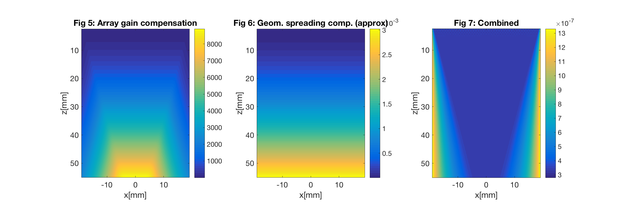
Now, let us investigate the weighting compensation a bit. Fig 5 shows the weighting calculated to compensate for the variable array gain caused by the dynamic aperture (constant f#). Fig 6 shows the weighting to compensate for the loss because of geometrical spreading. Fig 7 showns the combined weighting that is applied to the image.

Lateral lines through grid

[dummy,la_line_1] = min(abs(sca.z_axis - 5/1000));
[dummy,la_line_2] = min(abs(sca.z_axis - 25/1000));
[dummy,la_line_3] = min(abs(sca.z_axis - 45/1000));

f3 = figure(3);clf;
set(f3,'Position',[136 106 1026 697]);
subplot(321);hold all;
plot(sca.x_axis*1000,image.all{1}(la_line_1,:),'LineWidth',2,'DisplayName',image.tags{1} ,'Color','r')
plot(sca.x_axis*1000,image.all{2}(la_line_1,:),'LineWidth',2,'DisplayName',image.tags{2} ,'Color','b')
grid on; ylim([-65 0]); legend('location','nw'); title('Fig 8: Lateral line at z = 5mm');
xlabel('x[mm]');ylabel('Amplitude[dB]');set(gca,'FontSize',15);
subplot(322);hold all;
plot(sca.x_axis*1000,image.all{3}(la_line_1,:),'LineWidth',2,'DisplayName',image.tags{3} )
plot(sca.x_axis*1000,image.all{4}(la_line_1,:),'LineWidth',2,'DisplayName',image.tags{4} )
grid on; ylim([-65 0]); legend('location','sw'); title('Fig 9: Lateral line at z = 5mm');
xlabel('x[mm]');ylabel('Amplitude[dB]');set(gca,'FontSize',15);
subplot(323);hold all;
plot(sca.x_axis*1000,image.all{1}(la_line_2,:),'LineWidth',2,'DisplayName',image.tags{1} ,'Color','r')
plot(sca.x_axis*1000,image.all{2}(la_line_2,:),'LineWidth',2,'DisplayName',image.tags{2} ,'Color','b')
grid on; ylim([-65 0]); legend('location','sw'); title('Fig 10: Lateral line at z = 25mm');
xlabel('x[mm]');ylabel('Amplitude[dB]');set(gca,'FontSize',15);
subplot(324);hold all;
plot(sca.x_axis*1000,image.all{3}(la_line_2,:),'LineWidth',2,'DisplayName',image.tags{3} )
plot(sca.x_axis*1000,image.all{4}(la_line_2,:),'LineWidth',2,'DisplayName',image.tags{4} )
grid on; ylim([-65 0]); legend('location','sw'); title('Fig 11: Lateral line at z = 25mm');
xlabel('x[mm]');ylabel('Amplitude[dB]');set(gca,'FontSize',15);
subplot(325);hold all;
plot(sca.x_axis*1000,image.all{1}(la_line_3,:),'LineWidth',2,'DisplayName',image.tags{1} ,'Color','r')
plot(sca.x_axis*1000,image.all{2}(la_line_3,:),'LineWidth',2,'DisplayName',image.tags{2} ,'Color','b')
grid on; ylim([-65 0]); legend('location','sw'); title('Fig 12: Lateral line at z = 45mm');
xlabel('x[mm]');ylabel('Amplitude[dB]');set(gca,'FontSize',15);
subplot(326);hold all;
plot(sca.x_axis*1000,image.all{3}(la_line_3,:),'LineWidth',2,'DisplayName',image.tags{3})
plot(sca.x_axis*1000,image.all{4}(la_line_3,:),'LineWidth',2,'DisplayName',image.tags{4} )
grid on; ylim([-65 0]); legend('location','sw'); title('Fig 13: Lateral line at z = 45mm');
xlabel('x[mm]');ylabel('Amplitude[dB]');set(gca,'FontSize',15);

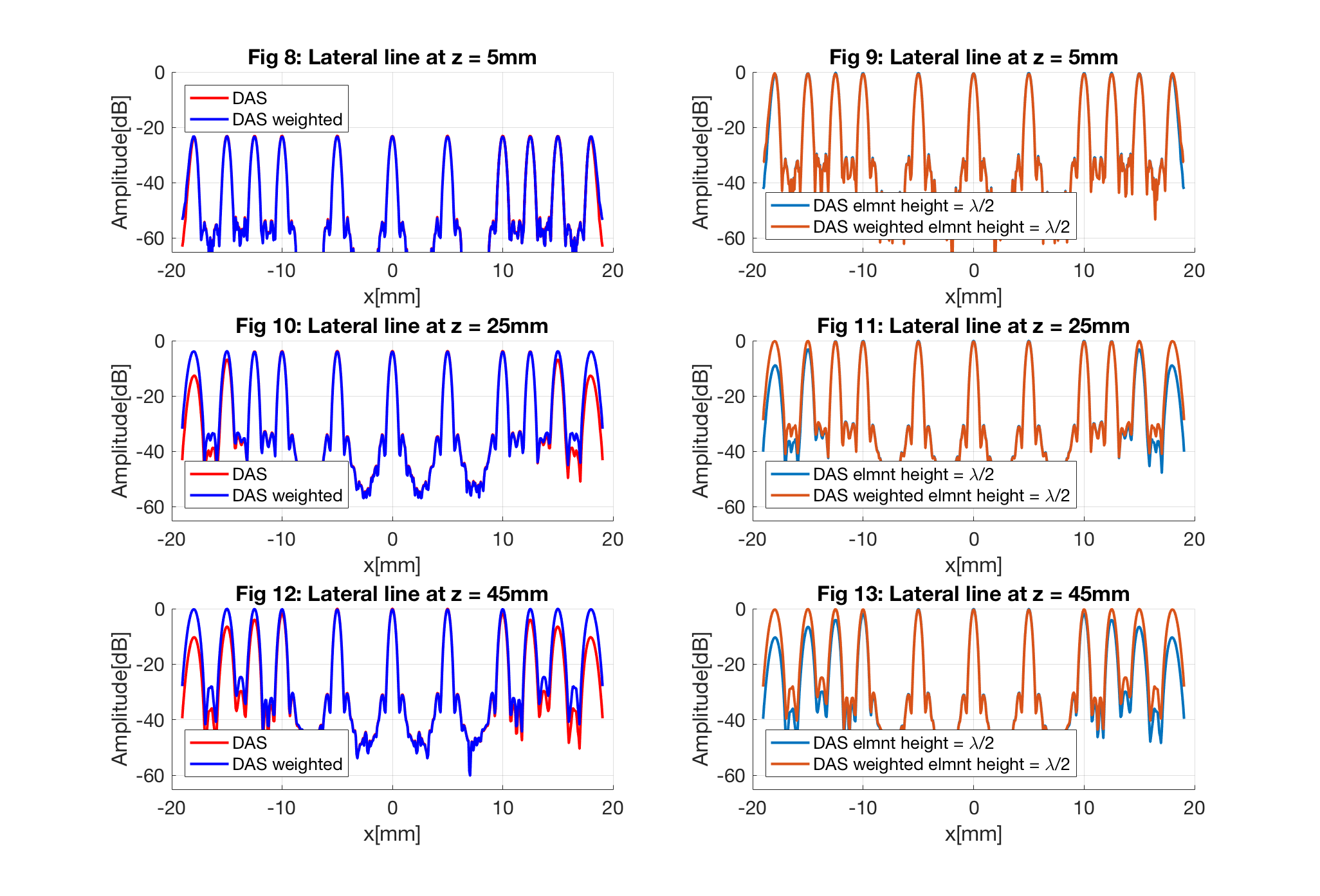
Yes, it was a bit hard to actually see the differences in intensity in Fig 1-4, so we have plotted the lateral line at z = 5 mm (Fig 8), z = 25 mm (Fig 10) and z = 45 mm (Fig 12) for the DAS images from the simulation non-omnidirectional elements both with and without the compensational weighting. And the lateral line at z = 5 mm (Fig 9), z = 25 mm (Fig 11) and z = 45 mm (Fig 13) for the DAS images from the omnidirectional elements with and withouth the compensational weighting.

From these figures, we can clearly see our observation from earlier, that the compensational weighting seems to compensate for the drop in amplitude towards the side of the image, while using omnidirectional weights compensate for the range dependent drop.

Axial lines through grid

[dummy,ax_line_1] = min(abs(sca.x_axis - -18/1000));
[dummy,ax_line_2] = min(abs(sca.x_axis - 0/1000));
[dummy,ax_line_3] = min(abs(sca.x_axis - 18/1000));

f4 = figure(4);clf;
set(f4,'Position',[136 106 1026 697]);
subplot(321);hold all;
plot(sca.x_axis*1000,image.all{1}(:,ax_line_1),'LineWidth',2,'DisplayName',image.tags{1},'Color','r','Marker','*')
plot(sca.x_axis*1000,image.all{2}(:,ax_line_1),'LineWidth',2,'DisplayName',image.tags{2},'Color','b')
grid on; ylim([-80 0]); legend('location','nw'); title('Fig 14: Axial line at x = -18mm');
xlabel('z[mm]');ylabel('Amplitude[dB]');set(gca,'FontSize',15);
subplot(322);hold all;
plot(sca.x_axis*1000,image.all{3}(:,ax_line_1),'LineWidth',2,'DisplayName',image.tags{3},'Marker','*')
plot(sca.x_axis*1000,image.all{4}(:,ax_line_1),'LineWidth',2,'DisplayName',image.tags{4})
grid on; ylim([-80 0]); legend('location','sw'); title('Fig 15: Axial line at x = -18mm');
xlabel('z[mm]');ylabel('Amplitude[dB]');set(gca,'FontSize',15);
subplot(323);hold all;
plot(sca.x_axis*1000,image.all{1}(:,ax_line_2),'LineWidth',2,'DisplayName',image.tags{1},'Color','r','Marker','*')
plot(sca.x_axis*1000,image.all{2}(:,ax_line_2),'LineWidth',2,'DisplayName',image.tags{2},'Color','b')
grid on; ylim([-80 0]); legend('location','sw'); title('Fig 16: Axial line at x = 0mm');
xlabel('z[mm]');ylabel('Amplitude[dB]');set(gca,'FontSize',15);
subplot(324);hold all;
plot(sca.x_axis*1000,image.all{3}(:,ax_line_2),'LineWidth',2,'DisplayName',image.tags{3},'Marker','*')
plot(sca.x_axis*1000,image.all{4}(:,ax_line_2),'LineWidth',2,'DisplayName',image.tags{4})
grid on; ylim([-80 0]); legend('location','sw'); title('Fig 17:Axial line at x = 0mm');
xlabel('z[mm]');ylabel('Amplitude[dB]');set(gca,'FontSize',15);
subplot(325);hold all;
plot(sca.x_axis*1000,image.all{1}(:,ax_line_3),'LineWidth',2,'DisplayName',image.tags{1},'Color','r','Marker','*')
plot(sca.x_axis*1000,image.all{2}(:,ax_line_3),'LineWidth',2,'DisplayName',image.tags{2},'Color','b')
grid on; ylim([-80 0]); legend('location','sw'); title('Fig 18: Axial line at x = 18mm');
xlabel('z[mm]');ylabel('Amplitude[dB]');set(gca,'FontSize',15);
subplot(326);hold all;
plot(sca.x_axis*1000,image.all{3}(:,ax_line_3),'LineWidth',2,'DisplayName',image.tags{3},'Marker','*')
plot(sca.x_axis*1000,image.all{4}(:,ax_line_3),'LineWidth',2,'DisplayName',image.tags{4})
grid on; ylim([-80 0]); legend('location','sw'); title('Fig 19: Axial line at x = 18mm');
xlabel('z[mm]');ylabel('Amplitude[dB]');set(gca,'FontSize',15);

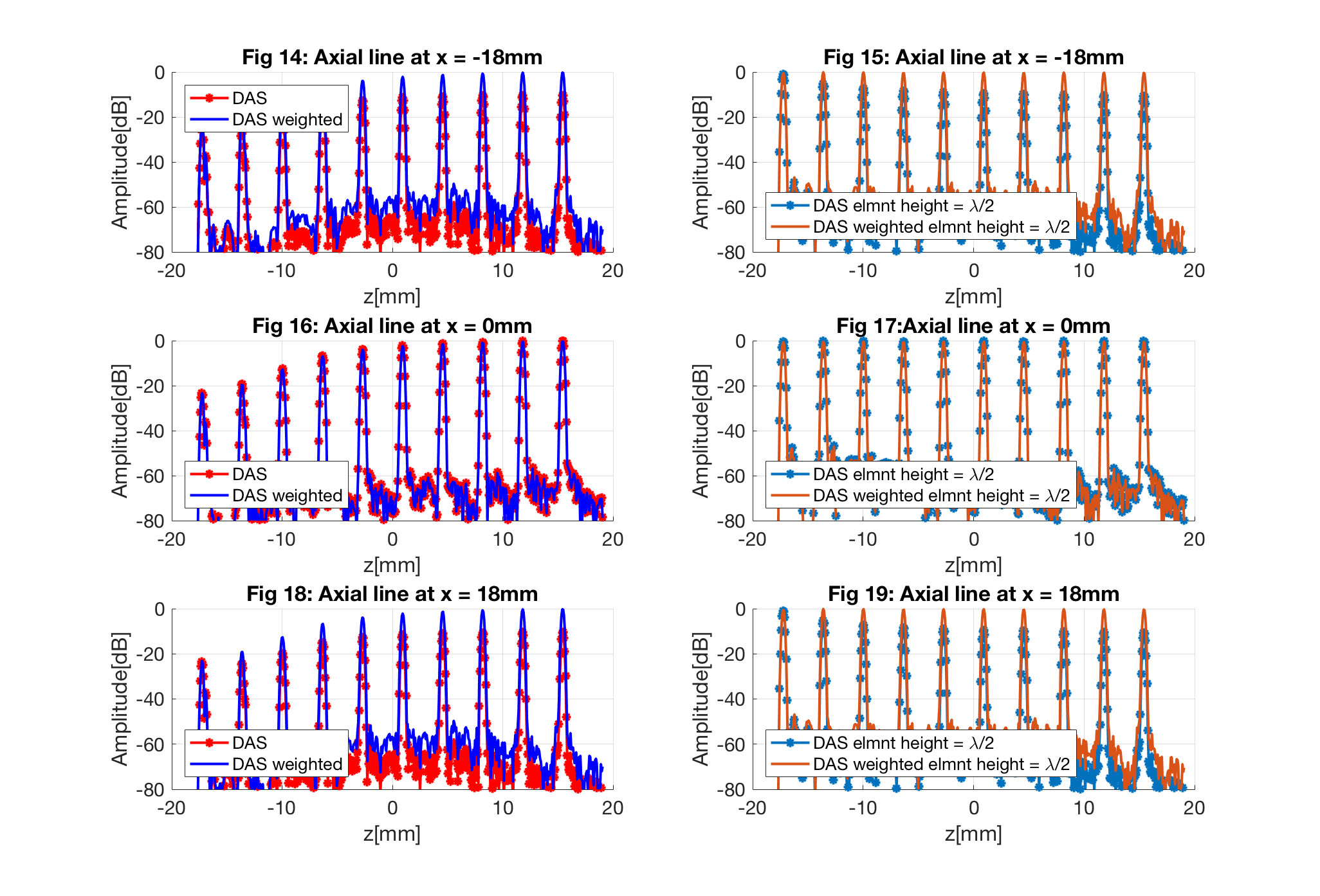
A better illustration of the range dependent drop in intensity for the images from the non-omnidirectional images is seen when we plot the axial line. Fig 14, 16 and 18 is from the non-omnidirectional elements. While Fig 15, 17 and 19 is the from the omnidirectional elements.

Scatter plot of intensity

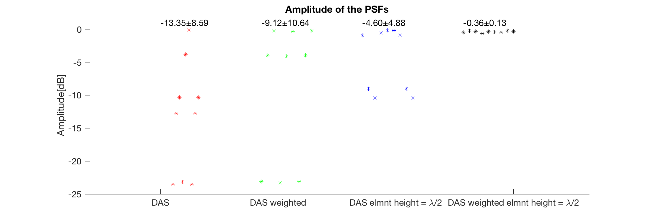
Lastly, we can plot the amplitude at some of the points as a scatter plot, to verify that DAS with weighting and omnidirectional elements gives uniform amplitude.

v_1 = image.all{1}([la_line_1 la_line_2 la_line_3],[ax_line_1 ax_line_2 ax_line_3]);
v_2 = image.all{2}([la_line_1 la_line_2 la_line_3],[ax_line_1 ax_line_2 ax_line_3]);
v_3 = image.all{3}([la_line_1 la_line_2 la_line_3],[ax_line_1 ax_line_2 ax_line_3]);
v_4 = image.all{4}([la_line_1 la_line_2 la_line_3],[ax_line_1 ax_line_2 ax_line_3]);

nbr_scatterers = length(v_1(:));
f5 = figure(5); hold all
set(f5,'Position',[81 428 1102 370])
plot(linspace(0.75,1.25,nbr_scatterers),v_1(:),'r*')
plot(linspace(2.5,3.5,nbr_scatterers),v_2(:),'g*')
plot(linspace(4.5,5.5,nbr_scatterers),v_3(:),'b*')
plot(linspace(6.5,7.5,nbr_scatterers),v_4(:),'k*')
set(gca,'XLim',[-1 9],'XTick',linspace(0.5,7.5,4))
ylim([-25 2])
xticklabels({image.tags{1},image.tags{2},image.tags{3},image.tags{4}})
text(0.5,1,sprintf(['%.2f' char(177) '%.2f'],mean(v_1(:)),std(v_1(:))),'FontSize',15)
text(2.5,1,sprintf(['%.2f' char(177) '%.2f'],mean(v_2(:)),std(v_2(:))),'FontSize',15)
text(4.5,1,sprintf(['%.2f' char(177) '%.2f'],mean(v_3(:)),std(v_3(:))),'FontSize',15)
text(6.5,1,sprintf(['%.2f' char(177) '%.2f'],mean(v_4(:)),std(v_4(:))),'FontSize',15)
ylabel('Amplitude[dB]');set(gca,'FontSize',15);
title('Amplitude of the PSFs');

Investigate for unform FOV for speckle from STAI imaging

We'll load some channel data from a speckle simulation from omnidirectional elements to verify that our observations from the grid is also true for speckle.

% Load the data and beamform the image by just interchanging the channel
% data object in the mid process.
channel_data_speckle = uff.channel_data();
channel_data_speckle.read([data_path filesep filename],'/channel_data_speckle');
mid.channel_data = channel_data_speckle;
b_data_speckle = mid.go();

UFF: reading channel_data_speckle [uff.channel_data]
UFF: reading sequence [uff.wave] [====================] 100%
uff.apodization: Inputs and outputs are unchanged. Skipping process.
USTB General beamformer MEX v1.1.2 .............done!

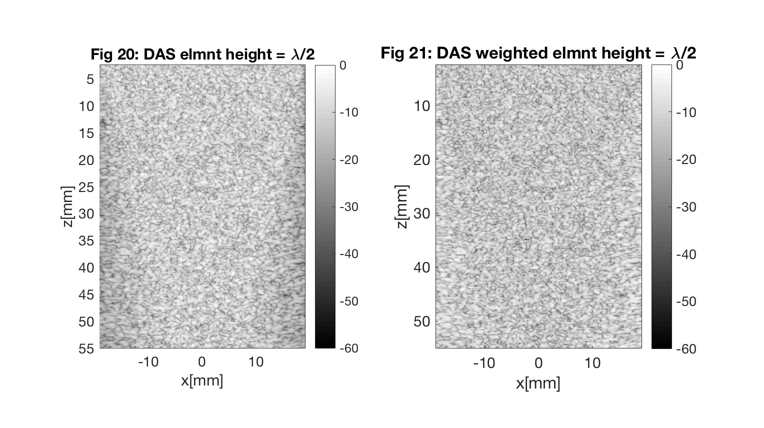
Multiply one image with the same weighting as earlier. The unweighted image is in Fig 20, while the weighted image is in Fig 21. We can see that the observation from earlier seems to be correct, that the combination of omnidirectional elements and compensation weighting gives a uniform FOV.

img_speckle = b_data_speckle.get_image('none');
img_speckle_weighted = img_speckle.*weights;
image_speckle.all{1} = db(abs(img_speckle./max(img_speckle(:))));
image_speckle.tags{1} = 'Fig 20: DAS elmnt height = \lambda/2';
image_speckle.all{2} = db(abs(img_speckle_weighted./max(img_speckle_weighted(:))));
image_speckle.tags{2} = 'Fig 21: DAS weighted elmnt height = \lambda/2';

f6 = figure(6);hold on;
set(f6,'Position',[419 370 764 428]);
b_data_speckle.plot(subplot(1,2,1),image_speckle.tags{1});

subplot(1,2,2)
imagesc(sca.x_axis*1000,sca.z_axis*1000,image_speckle.all{2});
colorbar;
colormap gray; caxis([-60 0]); axis image;
title(image_speckle.tags{2});xlabel('x[mm]');ylabel('z[mm]')
set(gca,'FontSize',15)

Plot lateral and axial lines.

f12 = figure(12);clf;
set(f12,'Position',[332 171 668 634]);
subplot(311);hold all;
plot(sca.x_axis*1000,image_speckle.all{1}(la_line_1,:),'LineWidth',2,'DisplayName',image_speckle.tags{1} ,'Color','r')
plot(sca.x_axis*1000,image_speckle.all{2}(la_line_1,:),'LineWidth',2,'DisplayName',image_speckle.tags{2} ,'Color','b')
grid on; ylim([-35 0]); legend('location','sw'); title('Fig 22: Lateral line at z = 5mm');
xlabel('x[mm]');ylabel('Amplitude[dB]');set(gca,'FontSize',15);
subplot(312);hold all;
plot(sca.x_axis*1000,image_speckle.all{1}(la_line_2,:),'LineWidth',2,'DisplayName',image_speckle.tags{1} ,'Color','r')
plot(sca.x_axis*1000,image_speckle.all{2}(la_line_2,:),'LineWidth',2,'DisplayName',image_speckle.tags{2} ,'Color','b')
grid on; ylim([-35 0]); legend('location','sw'); title('Fig 23: Lateral line at z = 25mm');
xlabel('x[mm]');ylabel('Amplitude[dB]');set(gca,'FontSize',15);
subplot(313);hold all;
plot(sca.x_axis*1000,image_speckle.all{1}(la_line_3,:),'LineWidth',2,'DisplayName',image_speckle.tags{1} ,'Color','r')
plot(sca.x_axis*1000,image_speckle.all{2}(la_line_3,:),'LineWidth',2,'DisplayName',image_speckle.tags{2} ,'Color','b')
grid on; ylim([-35 0]); legend('location','sw'); title('Fig 24: Lateral line at z = 45mm');
xlabel('x[mm]');ylabel('Amplitude[dB]');set(gca,'FontSize',15);

f13 = figure(13);clf;
set(f13,'Position',[332 171 668 634]);
subplot(311);hold all;
plot(sca.x_axis*1000,image_speckle.all{1}(:,ax_line_1),'LineWidth',2,'DisplayName',image_speckle.tags{1},'Color','r')
plot(sca.x_axis*1000,image_speckle.all{2}(:,ax_line_1),'LineWidth',2,'DisplayName',image_speckle.tags{2},'Color','b')
grid on; ylim([-35 0]); legend('location','sw'); title('Fig 25: Axial line at x = -18mm');
xlabel('z[mm]');ylabel('Amplitude[dB]');set(gca,'FontSize',15);
subplot(312);hold all;
plot(sca.x_axis*1000,image_speckle.all{1}(:,ax_line_2),'LineWidth',2,'DisplayName',image_speckle.tags{1},'Color','r')
plot(sca.x_axis*1000,image_speckle.all{2}(:,ax_line_2),'LineWidth',2,'DisplayName',image_speckle.tags{2},'Color','b')
grid on; ylim([-35 0]); legend('location','sw'); title('Fig 26: Axial line at x = 0mm');
xlabel('z[mm]');ylabel('Amplitude[dB]');set(gca,'FontSize',15);
subplot(313);hold all;
plot(sca.x_axis*1000,image_speckle.all{1}(:,ax_line_3),'LineWidth',2,'DisplayName',image_speckle.tags{1},'Color','r')
plot(sca.x_axis*1000,image_speckle.all{2}(:,ax_line_3),'LineWidth',2,'DisplayName',image_speckle.tags{2},'Color','b')
grid on; ylim([-35 0]); legend('location','sw'); title('Fig 27: Axial line at x = 18mm');
xlabel('z[mm]');ylabel('Amplitude[dB]');set(gca,'FontSize',15);

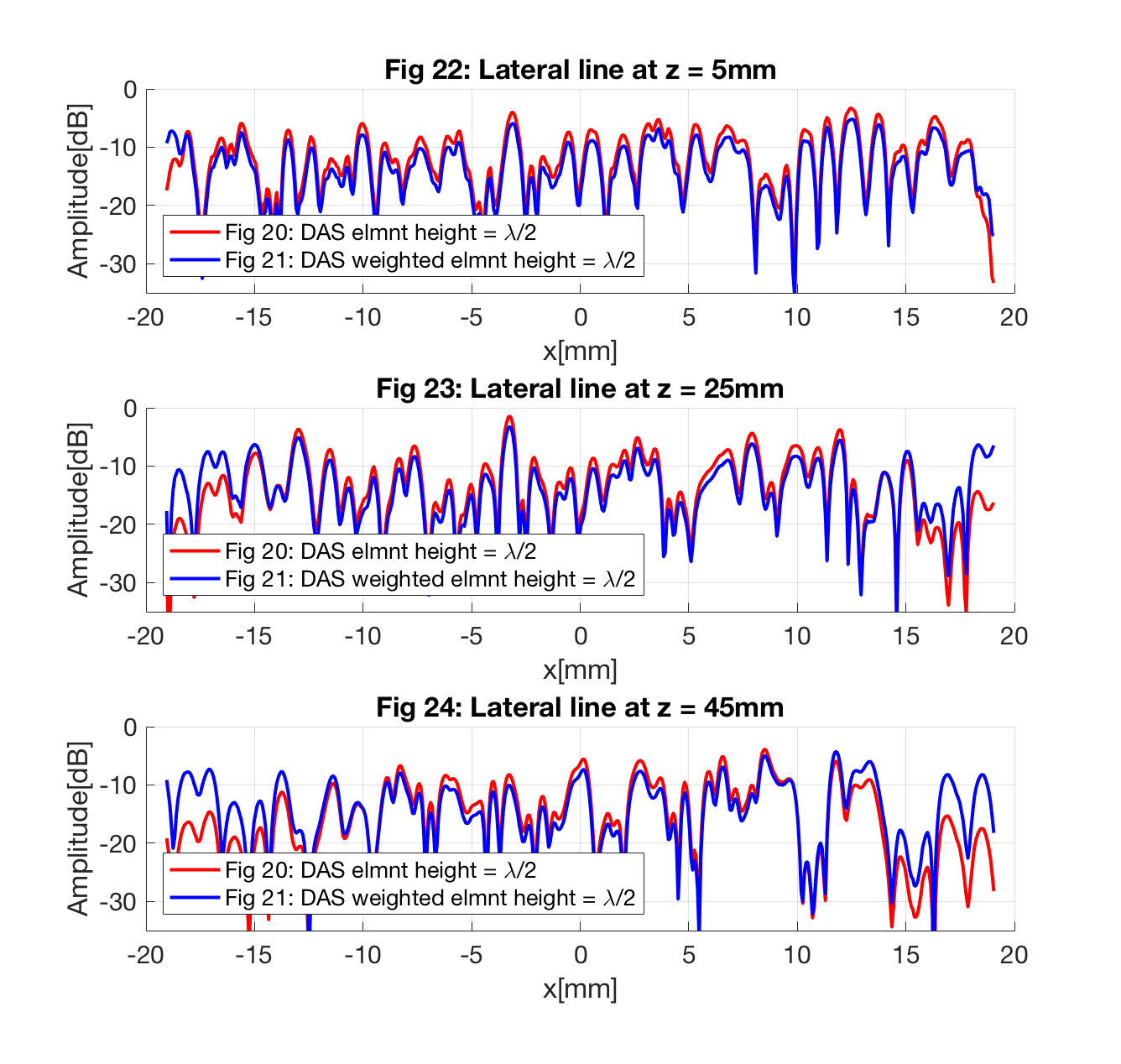
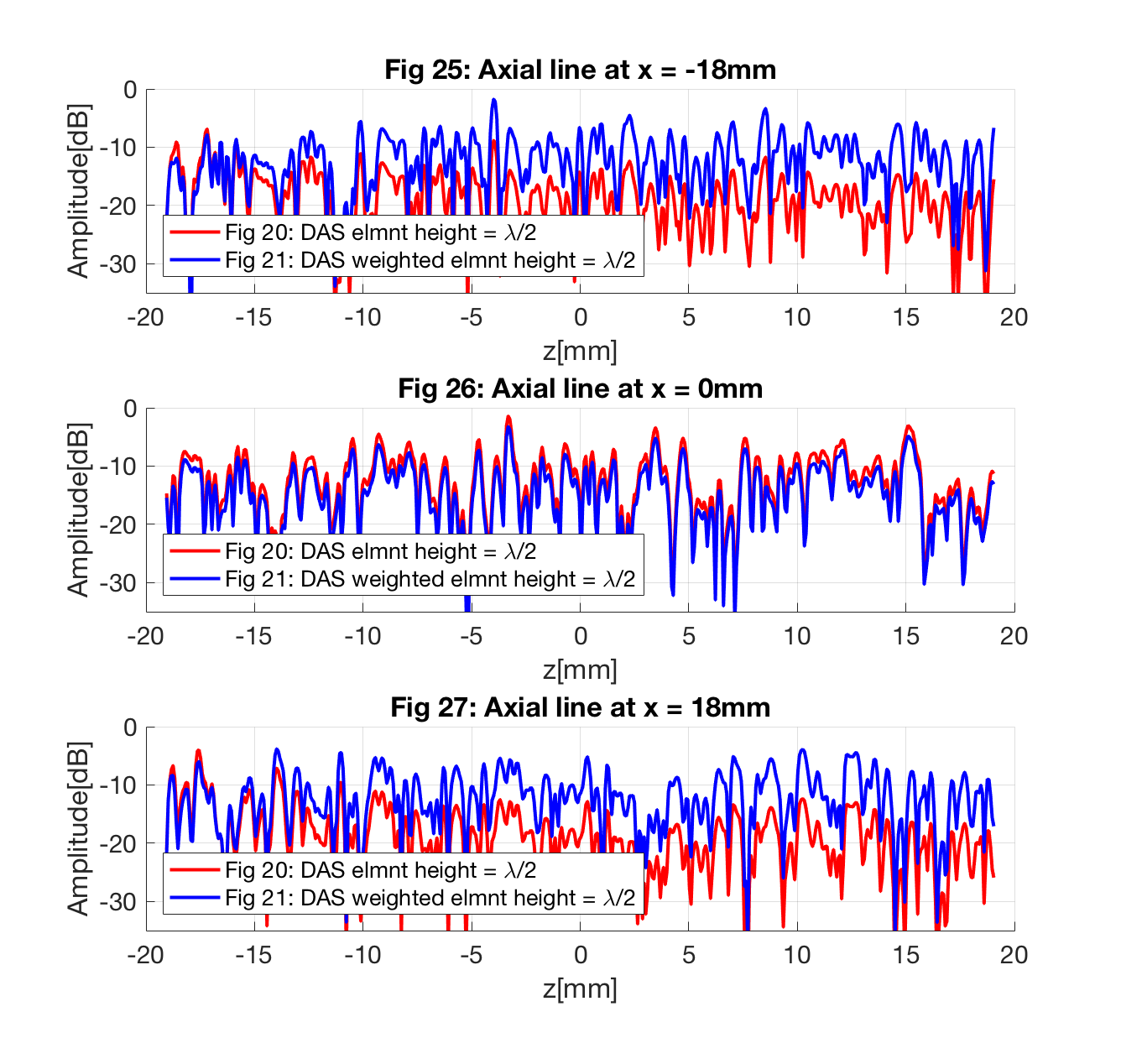
The lateral lines plotted in Fig 22-24 and the axial lines plotted in Fig 25-27 confirmes that omnidirectional elements and compensation weighting gives a uniform FOV.

Plot the estimated probability density of the speckle amplitude and compare to theoretically predicted Rayleigh distribution

envelope = abs(img_speckle);
envelope = envelope./max(envelope(:));
envelope_weighted = abs(img_speckle_weighted);
envelope_weighted = envelope_weighted./max(envelope_weighted(:));

m = mean(envelope(:));
s = std(envelope(:));
m_w = mean(envelope_weighted(:));
s_w = std(envelope_weighted(:));

snr_calculated_das = m/s
snr_calculated_das_weighted = m_w/s_w
snr_theoretical = (pi/(4-pi))^(1/2)
b = s/(sqrt((4-pi)/2)); %Scale parameter
b_w = s_w/(sqrt((4-pi)/2)); %Scale parameter

% Estimate PDF
x_axis = linspace(0,1,200);
[pdf_envelope,xout_1] = hist(envelope(:),x_axis);
pdf_envelope = pdf_envelope/sum(pdf_envelope)/(xout_1(2)-xout_1(1));
[pdf_envelope_weighted,xout] = hist(envelope_weighted(:),x_axis);
pdf_envelope_weighted = pdf_envelope_weighted/sum(pdf_envelope_weighted)/(xout(2)-xout(1));

% Theoretical Rayleigh PDF
theoretical_pdf = (x_axis./b^2).*exp(-x_axis.^2/(2.*b^2));
theoretical_pdf_weighted = (x_axis./b_w^2).*exp(-x_axis.^2/(2.*b_w^2));

color=[0.5 1 0.5];
figure(2);clf;
plot(xout_1,pdf_envelope,'LineWidth',2,'Color','b','DisplayName','Estimated PDF');hold on;
plot(x_axis,theoretical_pdf,'-*','Color','b','LineWidth',2,'DisplayName','Rayleigh Theoretical PDF');
plot(xout,pdf_envelope_weighted,'LineWidth',2,'Color','r','DisplayName','Estimated PDF weighted');hold on;
plot(x_axis,theoretical_pdf_weighted,'-*','Color','r','LineWidth',2,'DisplayName','Rayleigh Theoretical PDF');

title('Fig 28: PDF of envelope');
xlabel('Normalized amplitude');
ylabel('Probability')
legend('show');

snr_calculated_das =

  single

    1.7096


snr_calculated_das_weighted =

  single

    1.8754


snr_theoretical =

    1.9131

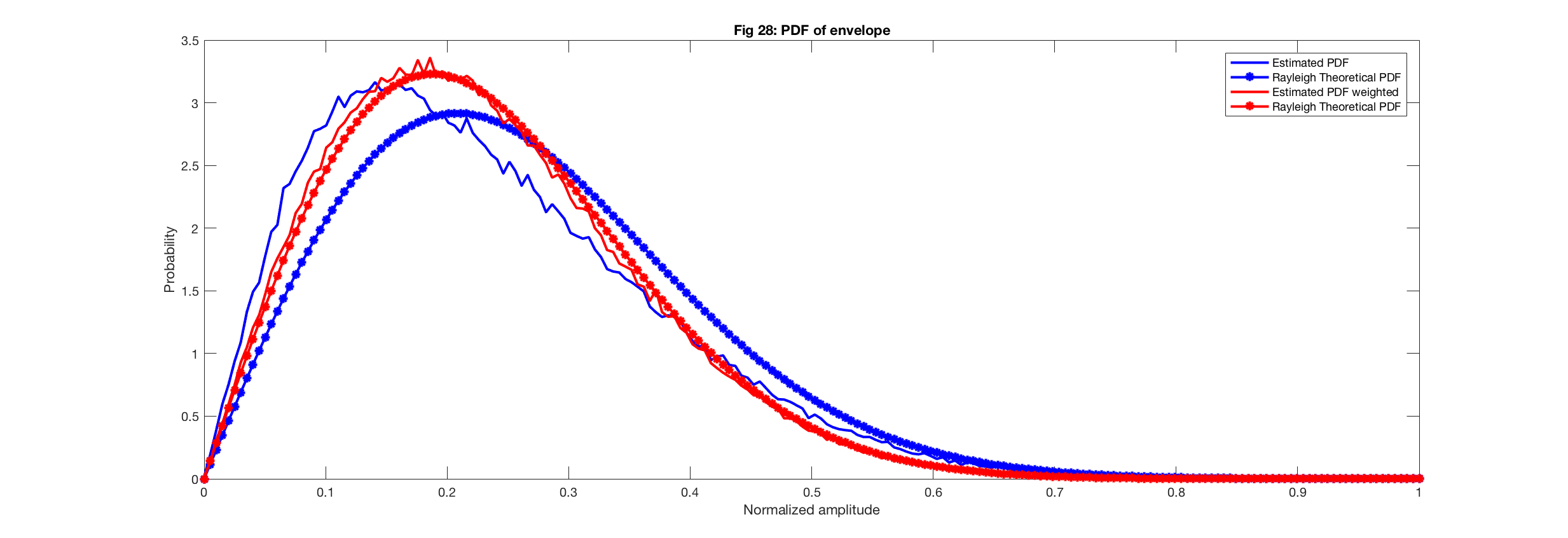
Lastly, in Fig we have plotted the estimated PDF of both speckle images, both with and without weighting, and compare it to the teoretically predicted Rayleig distribution. We can clearly see that the estimted PDF from the DAS image with compensation weighting fits much better with the theoretical distribution than DAS without weighting. We can also se that the calculted SNR is much closer to the theoretival 1.91 for the DAS with weighting, 1.88, compared to DAS withouth weighting 1.71.

Published with MATLAB® R2016b