CPWC simulation to compare speeds of the various USTB beamformers.

Contents

In this example, we conduct a simple simulation to compare the speeds achieved with USTB's:

This tutorial assumes familiarity with the contents of the 'CPWC simulation with the USTB built-in Fresnel simulator' tutorial. Please feel free to refer back to that for more details.

by Alfonso Rodriguez-Molares alfonso.r.molares@ntnu.no and Arun Asokan Nair anair8@jhu.edu 16.05.2017

clear all;
close all;

Phantom

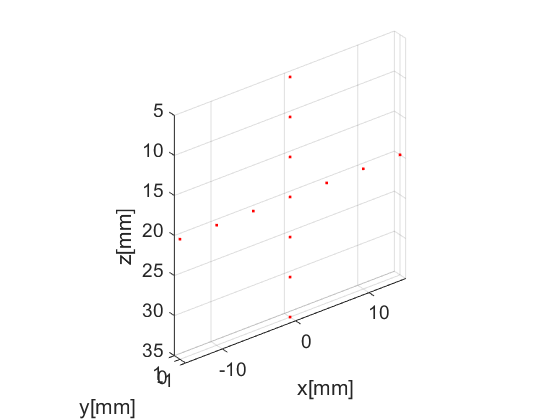
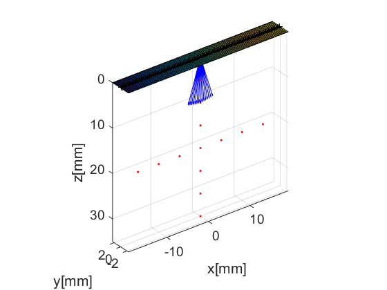
Our first step is to define an appropriate phantom structure as input. Our phantom here is simply a collection of point scatterers. USTB's implementation of phantom comes with a plot method for free!

x_sca=[zeros(1,7) -15e-3:5e-3:15e-3];
z_sca=[5e-3:5e-3:35e-3 20e-3*ones(1,7)];
N_sca=length(x_sca);
pha=uff.phantom();
pha.sound_speed=1540;            % speed of sound [m/s]
pha.points=[x_sca.', zeros(N_sca,1), z_sca.', ones(N_sca,1)];    % point scatterer position [m]
fig_handle=pha.plot();

Probe

The next step is to define the probe structure which contains information about the probe's geometry. This too comes with % a plot method that enables visualization of the probe with respect to the phantom. The probe we will use in our example is a linear array transducer with 128 elements.

prb=uff.linear_array();
prb.N=128;                  % number of elements
prb.pitch=300e-6;           % probe pitch in azimuth [m]
prb.element_width=270e-6;   % element width [m]
prb.element_height=5000e-6; % element height [m]
prb.plot(fig_handle);

Pulse

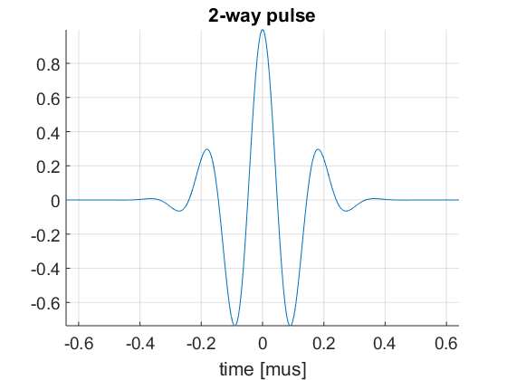
We then define the pulse-echo signal which is done here using the fresnel simulator's pulse structure. We could also use 'Field II' for a more accurate model.

pul=uff.pulse();
pul.center_frequency=5.2e6;       % transducer frequency [MHz]
pul.fractional_bandwidth=0.6;     % fractional bandwidth [unitless]
pul.plot([],'2-way pulse');

Sequence generation

Now, we shall generate our sequence! Keep in mind that the fresnel simulator takes the same sequence definition as the USTB beamformer. In UFF and USTB a sequence is defined as a collection of wave structures.

For our example here, we define a sequence of 15 plane-waves covering an angle span of radians. The wave structure has a plot method which plots the direction of the transmitted plane-wave.

N_plane_waves=15;
angles=linspace(-0.3,0.3,N_plane_waves);
seq=uff.wave();
for n=1:N_plane_waves
    seq(n)=uff.wave();
    seq(n).probe=prb;
    seq(n).source.azimuth=angles(n);
    seq(n).source.distance=Inf;
    seq(n).sound_speed=pha.sound_speed;

    % show source
    fig_handle=seq(n).source.plot(fig_handle);
end

The Fresnel simulator

Finally, we launch the built-in simulator. The simulator takes in a phantom, pulse, probe and a sequence of wave structures along with the desired sampling frequency, and returns a channel_data UFF structure.

sim=fresnel();

% setting input data
sim.phantom=pha;                % phantom
sim.pulse=pul;                  % transmitted pulse
sim.probe=prb;                  % probe
sim.sequence=seq;               % beam sequence
sim.sampling_frequency=41.6e6;  % sampling frequency [Hz]

% we launch the simulation. Go!
channel_data=sim.go();

USTB's Fresnel impulse response simulator (v1.0.5)
---------------------------------------------------------------

Scan

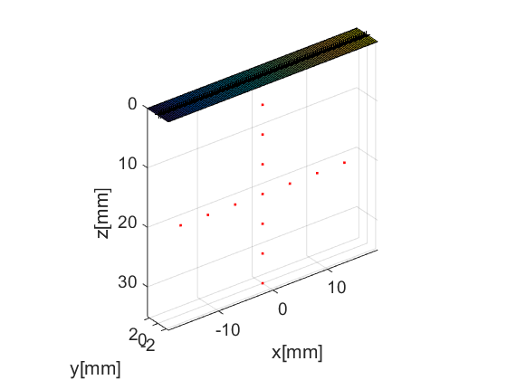
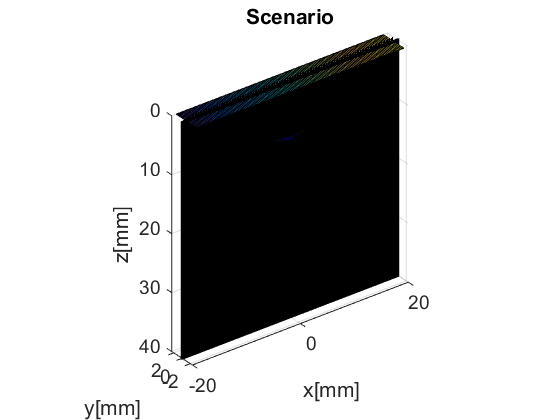
The scan area is defines as a collection of pixels spanning our region of interest. For our example here, we use the linear_scan structure, which is defined with just two axes. scan too has a useful plot method it can call.

sca=uff.linear_scan(linspace(-20e-3,20e-3,256).', linspace(0e-3,40e-3,256).');
sca.plot(fig_handle,'Scenario');    % show mesh

Beamformer

With channel_data and a scan we have all we need to produce an ultrasound image. We now use a USTB structure beamformer, that takes an apodization structure in addition to the channel_data and scan.

bmf=beamformer();
bmf.channel_data=channel_data;
bmf.scan=sca;

bmf.receive_apodization.window=uff.window.tukey50;
bmf.receive_apodization.f_number=1.0;
bmf.receive_apodization.apex.distance=Inf;

bmf.transmit_apodization.window=uff.window.tukey50;
bmf.transmit_apodization.f_number=1.0;
bmf.transmit_apodization.apex.distance=Inf;

The beamformer structure allows you to implement different beamformers by combination of multiple built-in processes. By changing the process chain other beamforming sequences can be implemented. It returns yet another UFF structure: beamformed_data.

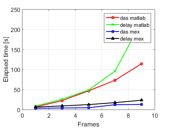
% To achieve the goal of this example, we combine 4 pairs of *processes*
% # *das_matlab* and % *coherent_compounding*
% # *delay_matlab* and % *coherent_compounding*
% # *das_mex* and % *coherent_compounding*
% # *delay_mex* and % *coherent_compounding*
% to produce coherently compounded images and examine each one's speed with
% respect to the others for increasing amounts of data.

% beamforming
n_frame=1:2:10
for n=1:length(n_frame)
    % replicate frames
    channel_data.data=repmat(channel_data.data(:,:,:,1),[1 1 1 n_frame(n)]);

    % Time USTB's MATLAB delay-and-sum implementation
    tic
    b_data=bmf.go({process.das_matlab() process.coherent_compounding()});
    das_matlab_time(n)=toc;

    % Time USTB's MATLAB delay implementation
    tic
    b_data=bmf.go({process.delay_matlab() process.coherent_compounding()});
    delay_matlab_time(n)=toc;

    % Time USTB's MEX delay-and-sum implementation
    tic
    b_data=bmf.go({process.das_mex() process.coherent_compounding()});
    das_mex_time(n)=toc;

    % Time USTB's MEX delay implementation
    tic
    b_data=bmf.go({process.delay_mex() process.coherent_compounding()});
    delay_mex_time(n)=toc;

    % Plot the runtimes
    figure(101);
    plot(n_frame(1:n),das_matlab_time(1:n),'ro-','linewidth',2); hold on; grid on;
    plot(n_frame(1:n),delay_matlab_time(1:n),'gx-','linewidth',2);
    plot(n_frame(1:n),das_mex_time(1:n),'bs-','linewidth',2);
    plot(n_frame(1:n),delay_mex_time(1:n),'k^-','linewidth',2);
    legend('das matlab','delay matlab','das mex','delay mex');
    xlabel('Frames');
    ylabel('Elapsed time [s]');
    set(gca,'fontsize',14)
end

n_frame =

     1     3     5     7     9

Published with MATLAB® R2015a