CPWC (low-resolution) simulation with the USTB built-in Fresnel simulator

In this example we show how to use the built-in fresnel simulator in USTB to generate a Coherent Plane-Wave Compounding (CPWC) dataset and how it can be beamformed with USTB.

Related materials:

Montaldo et al. 2009

This tutorial assumes familiarity with the contents of the 'CPWC simulation with the USTB built-in Fresnel simulator' tutorial. Please feel free to refer back to that for more details.

by Alfonso Rodriguez-Molares alfonso.r.molares@ntnu.no and Arun Asokan Nair anair8@jhu.edu 16.05.2017

Phantom
Probe
Pulse
Sequence generation
The Fresnel simulator
Scan
Beamformer

Phantom

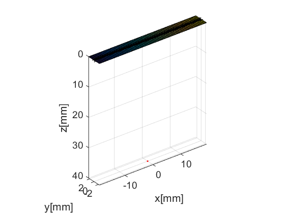
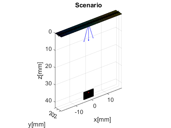
Our first step is to define an appropriate phantom structure as input. Our phantom here is simply a single point scatterer. USTB's implementation of phantom comes with a plot method for free!

pha=uff.phantom();
pha.sound_speed=1540;            % speed of sound [m/s]
pha.points=[0,  0, 40e-3, 1];    % point scatterer position [m]
fig_handle=pha.plot();

Probe

Another UFF structure is probe. You've guessed it, it contains information about the probe's geometry. USTB's implementation comes with a plot method. When combined with the previous Figure we can see the position of the probe respect to the phantom.

prb=uff.linear_array();
prb.N=128;                  % number of elements
prb.pitch=300e-6;           % probe pitch in azimuth [m]
prb.element_width=270e-6;   % element width [m]
prb.element_height=5000e-6; % element height [m]
prb.plot(fig_handle);

Pulse

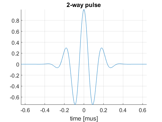
We then define the pulse-echo signal which is done here using the fresnel simulator's pulse structure. We could also use 'Field II' for a more accurate model.

pul=uff.pulse();
pul.center_frequency=5.2e6;       % transducer frequency [MHz]
pul.fractional_bandwidth=0.6;     % fractional bandwidth [unitless]
pul.plot([],'2-way pulse');

Sequence generation

Now, we shall generate our sequence! Keep in mind that the fresnel simulator takes the same sequence definition as the USTB beamformer. In UFF and USTB a sequence is defined as a collection of wave structures.

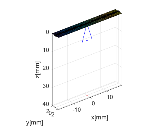
For our example here, we define a sequence of 3 plane-waves covering an angle span of $[-0.3, 0.3]$ radians. The wave structure has a plot method which plots the direction of the transmitted plane-wave.

N=3;                           % number of plane waves
angles=linspace(-0.3,0.3,N);    % angle vector [rad]
seq=uff.wave();
for n=1:N
    seq(n)=uff.wave();

    seq(n).source.azimuth=angles(n);
    seq(n).source.distance=Inf;

    seq(n).probe=prb;

    seq(n).sound_speed=pha.sound_speed;

    % show source
    fig_handle=seq(n).source.plot(fig_handle);
end

The Fresnel simulator

Finally, we launch the built-in simulator. The simulator takes in a phantom, pulse, probe and a sequence of wave structures along with the desired sampling frequency, and returns a channel_data UFF structure.

sim=fresnel();

% setting input data
sim.phantom=pha;                % phantom
sim.pulse=pul;                  % transmitted pulse
sim.probe=prb;                  % probe
sim.sequence=seq;               % beam sequence
sim.sampling_frequency=41.6e6;  % sampling frequency [Hz]

% we launch the simulation. Go!
channel_data=sim.go();

USTB's Fresnel impulse response simulator (v1.0.5)
---------------------------------------------------------------

Scan

The scan area is defines as a collection of pixels spanning our region of interest. For our example here, we use the linear_scan structure, which is defined with just two axes. scan too has a useful plot method it can call.

sca=uff.linear_scan(linspace(-3e-3,3e-3,200).', linspace(39e-3,43e-3,200).');
sca.plot(fig_handle,'Scenario');    % show mesh

Beamformer

With channel_data and a scan we have all we need to produce an ultrasound image. We now use a USTB structure beamformer, that takes an apodization structure in addition to the channel_data and scan.

bmf=beamformer();
bmf.channel_data=channel_data;
bmf.scan=sca;

bmf.receive_apodization.window=uff.window.tukey50;
bmf.receive_apodization.f_number=1.7;
bmf.receive_apodization.apex.distance=Inf;

% Setting transmit apodization to "none" since we want to look at the
% individual low quality PW's
bmf.transmit_apodization.window=uff.window.none;

The beamformer structure allows you to implement different beamformers by combination of multiple built-in processes. By changing the process chain other beamforming sequences can be implemented. It returns yet another UFF structure: beamformed_data.

% To achieve the goal of this example, we only use delay-and-sum (
% implemented in the *das_matlab()* process) and not coherent compounding
% as we want to output the low quality PW images each formed from only one
% plane wave transmission.

b_data=bmf.go({process.das_matlab()});

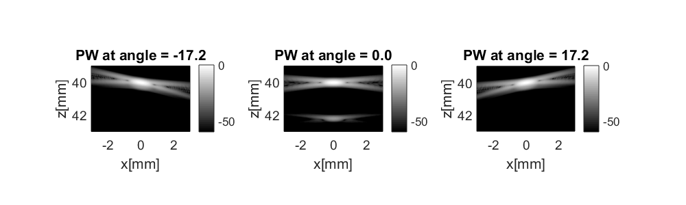
Finally, display each individual low quality plane wave image. Fin!

figure('Position',[100 100 1000 300])
h1 = subplot(1,3,1);
angle_1 = rad2deg(channel_data.sequence(1,1).source.azimuth);
b_data(1,1).plot(h1,sprintf('PW at angle = %0.1f',angle_1));

h2 = subplot(1,3,2);
angle_2 = rad2deg(channel_data.sequence(1,2).source.azimuth);
b_data(1,2).plot(h2,sprintf('PW at angle = %0.1f',angle_2));

h3 = subplot(1,3,3);
angle_3 = rad2deg(channel_data.sequence(1,3).source.azimuth);
b_data(1,3).plot(h3,sprintf('PW at angle = %0.1f',angle_3));