Delay Multiply And Sum on FI data from an UFF file

This script is also available as /publications/TUFFC/Prieur_et_al_Signal_coherence_and_image_amplitude_with_the_fDMAS /FI_UFF_FIeldII_simulations_Fig2_and_Fig3.m in the USTB repository.

Creating the simulated results in the paper:

F. Prieur, O. M. H. Rindal and A. Austeng, "Signal coherence and image amplitude with the Filtered-Delay-Multiply-And-Sum beamformer," in IEEE Transactions on Ultrasonics, Ferroelectrics, and Frequency Control. doi: 10.1109/TUFFC.2018.2831789

This script re-create Figs. 2 and 3 of the article.

This code uses the UltraSound ToolBox (USTB) and you'll need to download it first to successfully rund this code. To know more about the USTB visit http://www.ustb.no/

by Fabrice Prieur fabrice@ifi.uio.no 18.05.2018

Read data
Reading channel data from UFF file
Define Scan
Delay the channel data
Do DAS beamforming doing coherent compounding of delayed data
Create the DMAS image using the delay_multiply_and_sum postprocess
Get images
Speckle image
Speckle statistics

Read data

To read data from a UFF file the first we need is, you guessed it, a UFF file. We check if it is on the current path and download it from the USTB websever.

clear all; close all;

% data location
url='http://ustb.no/datasets/';      % if not found downloaded from here
local_path = [ustb_path(),'/data/']; % location of example data


% Choose dataset
filename='FieldII_speckle_simulation.uff';

% check if the file is available in the local path or downloads otherwise
tools.download(filename, url, local_path);

Reading channel data from UFF file

channel_data=uff.read_object([local_path filename],'/channel_data');

UFF: reading channel_data [uff.channel_data]
UFF: reading sequence [uff.wave] [====================] 100%

Print info about the dataset. If you want to use this dataset, you are welcome to, but please cite the refrence below.

channel_data.print_authorship

Name: 		 Field II simulation of well developed speckle. 
Reference: 	 F. Prieur, O. M. H. Rindal and A. Austeng,  
		 "Signal coherence and image amplitude with the  
		 Filtered-Delay-Multiply-And-Sum beamformer," in  
		 IEEE Transactions on Ultrasonics, Ferroelectrics,  
		 and Frequency Control. doi:  
		 10.1109/TUFFC.2018.2831789 
Author(s): 	 Ole Marius Hoel Rindal <olemarius@olemarius.net> 
		 Fabruce Prieur <fabrice@ifi.uio.no> 
Version: 	 1.1.1

Define Scan

Define the image coordinates we want to beamform in the scan object. Notice that we need to use quite a lot of samples in the z-direction. This is because the DMAS creates an "artificial" second harmonic signal, so we need high enough sampling frequency in the image to get a second harmonic signal.

z_axis = linspace(35e-3,45e-3,1200).';
x_axis = zeros(channel_data.N_waves,1);
for w = 1:channel_data.N_waves
   x_axis(w) = channel_data.sequence(w).source.x;
end

scan=uff.linear_scan('x_axis',x_axis,'z_axis',z_axis);

Delay the channel data

delay = midprocess.das();
delay.channel_data=channel_data;
delay.scan=scan;
delay.dimension = dimension.transmit();
delay.transmit_apodization.window=uff.window.scanline;

delay.receive_apodization.window=uff.window.none;
delay.receive_apodization.f_number=3;

delayed_b_data = delay.go();

USTB General beamformer MEX v1.1.2 .............done!

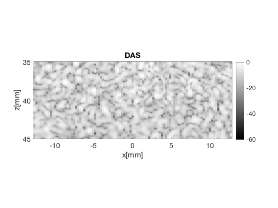
Do DAS beamforming doing coherent compounding of delayed data

disp('Beamforming data using DAS');
das = postprocess.coherent_compounding();
das.input = delayed_b_data;
b_data = das.go();

b_data.plot([],'DAS');

Beamforming data using DAS

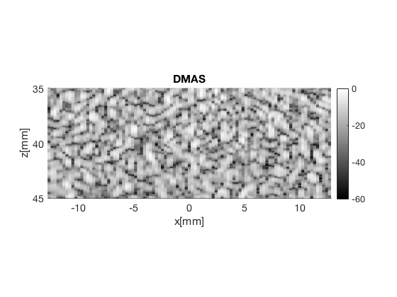
Create the DMAS image using the delay_multiply_and_sum postprocess

disp('Beamforming data using DMAS')
dmas = postprocess.delay_multiply_and_sum();
dmas.dimension = dimension.receive;
dmas.channel_data = channel_data;
dmas.input = delayed_b_data;
dmas.receive_apodization = delay.receive_apodization;

b_data_dmas=dmas.go();

b_data_dmas.plot(100,'DMAS');

Beamforming data using DMAS
Warning: Missing probe and apodization data; full aperture is assumed. 
Warning: If the result looks funky, you might need to tune the filter paramters
of DMAS using the filter_freqs property. Use the plot to check that everything
is OK.

Get images

imgDMAS=reshape(b_data_dmas.data,b_data_dmas.scan.N_z_axis,b_data_dmas.scan.N_x_axis);
imgDAS=reshape(b_data.data,b_data.scan.N_z_axis,b_data.scan.N_x_axis);

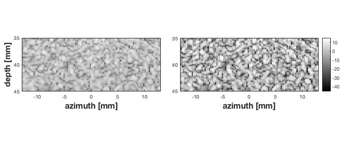
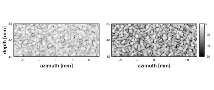
Speckle image

Image normalization by image mean

figure('color','w','position',[  -850   706   682   287],'name','norm mean');
subplot(1,2,1);
mDAS=mean(abs(imgDAS(:)));
imagesc(b_data.scan.x_axis*1e3,b_data.scan.z_axis*1e3,db(abs(imgDAS)/mDAS));
caxis([-45 15]);daspect([1 1 1]);set(gca,'position',[0.063 0.148 0.4 0.815]);
xlabel('azimuth [mm]','fontweight','bold','fontsize',16)
ylabel('depth [mm]','fontweight','bold','fontsize',16)
subplot(1,2,2);
mDMAS=mean(abs(imgDMAS(:)));
imagesc(b_data_dmas.scan.x_axis*1e3,b_data_dmas.scan.z_axis*1e3,db(abs(imgDMAS)/mDMAS));
caxis([-45 15]);colorbar;colormap gray;
set(gca,'position',[0.52 0.148 0.4 0.815]);daspect([1 1 1]);
xlabel('azimuth [mm]','fontweight','bold','fontsize',16)

% Image normalization by image max
figure('color','w','position',[  -850   706   682   287],'name','norm max');
subplot(1,2,1);
mDAS=max(abs(imgDAS(:)));
imagesc(b_data.scan.x_axis*1e3,b_data.scan.z_axis*1e3,db(abs(imgDAS)/mDAS));
caxis([-60 0]);daspect([1 1 1]);set(gca,'position',[0.063 0.148 0.4 0.815]);
xlabel('azimuth [mm]','fontweight','bold','fontsize',16)
ylabel('depth [mm]','fontweight','bold','fontsize',16)
subplot(1,2,2);
mDMAS=max(abs(imgDMAS(:)));
imagesc(b_data_dmas.scan.x_axis*1e3,b_data_dmas.scan.z_axis*1e3,db(abs(imgDMAS)/mDMAS));
caxis([-60 0]);colorbar;colormap gray;
set(gca,'position',[0.52 0.148 0.4 0.815]);daspect([1 1 1]);
xlabel('azimuth [mm]','fontweight','bold','fontsize',16)

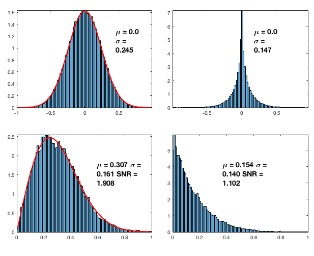
Speckle statistics

figure('color','w','position',[-616    62   617   502]);
subplot('position',[0.053 0.58 0.43 0.38]);
h=histogram(real(imgDAS(:)/mDAS),100,'Normalization','pdf');
x=h.BinEdges(1:end-1)+h.BinWidth/2;axis('tight')
sigma=std(imag(imgDAS(:)/mDAS));
mu=mean(imag(imgDAS(:)/mDAS));
a=annotation('textbox',[0.36 0.77 0.104 0.130],...
    'String',['\mu = ',num2str(mu,'%.1f'),' \sigma = ',num2str(sigma,'%.3f')]);
set(a,'linestyle','none','fontweight','bold','fontsize',14);
% Gaussian distribution
hold on;plot(x,exp(-x.^2/2/sigma^2)/sqrt(2*pi)/sigma,'r','linewidth',2);
axis('tight')
subplot('position',[0.053 0.094 0.43 0.38]);
h=histogram(abs(imgDAS(:)/mDAS),100,'Normalization','pdf');
x=h.BinEdges(1:end-1)+h.BinWidth/2;
% Rayleigh distribution
hold on;plot(x,x/sigma^2.*exp(-x.^2/2/sigma^2),'r','linewidth',2);
axis('tight')
sigma=std(abs(imgDAS(:)/mDAS));
mu=mean(abs(imgDAS(:)/mDAS));
a=annotation('textbox',[0.30 0.186 0.180 0.194],...
    'String',['\mu = ',num2str(mu,'%.3f'),...
    ' \sigma = ',num2str(sigma,'%.3f'),...
    ' SNR = ',num2str(mu/sigma,'%.3f')]);
set(a,'linestyle','none','fontweight','bold','fontsize',14);

subplot('position',[0.55 0.58 0.43 0.38]);
h=histogram(real(imgDMAS(:)/mDMAS),100,'Normalization','pdf');
axis('tight')
sigma=std(imag(imgDMAS(:)/mDMAS));
mu=mean(imag(imgDMAS(:)/mDMAS));
a=annotation('textbox',[0.8 0.77 0.104 0.130],...
    'String',['\mu = ',num2str(mu,'%.1f'),' \sigma = ',num2str(sigma,'%.3f')]);
set(a,'linestyle','none','fontweight','bold','fontsize',14);
subplot('position',[0.55 0.094 0.43 0.38]);
h=histogram(abs(imgDMAS(:)/mDMAS),100,'Normalization','pdf');
axis('tight')
sigma=std(abs(imgDMAS(:)/mDMAS));
mu=mean(abs(imgDMAS(:)/mDMAS));
a=annotation('textbox',[0.7 0.186 0.180 0.194],...
    'String',['\mu = ',num2str(mu,'%.3f'),...
    ' \sigma = ',num2str(sigma,'%.3f'),...
    ' SNR = ',num2str(mu/sigma,'%.3f')]);
set(a,'linestyle','none','fontweight','bold','fontsize',14);