Delay Multiply And Sum on FI data from an UFF file

This script is also available as /publications/TUFFC/Prieur_et_al_Signal_coherence_and_image_amplitude_with_the_fDMAS /FI_UFF_delay_multiply_and_sum_Fig5_and_Fig6.m in the USTB repository.

Create the images with the recorded channel data in the paper:

F. Prieur, O. M. H. Rindal and A. Austeng, "Signal coherence and image amplitude with the Filtered-Delay-Multiply-And-Sum beamformer," in IEEE Transactions on Ultrasonics, Ferroelectrics, and Frequency Control. doi: 10.1109/TUFFC.2018.2831789

This script re-create Figs. 5 and 6 of the article.

This code uses the UltraSound ToolBox (USTB) and you'll need to download it first to successfully rund this code. To know more about the USTB visit http://www.ustb.no/

by Ole Marius Hoel Rindal olemarius@olemarius.net 10.10.2017

Contents

Setting up file path

To read data from a UFF file the first we need is, you guessed it, a UFF file. We check if it is on the current path and download it from the USTB websever.

clear all; close all;

% data location
url='http://ustb.no/datasets/';      % if not found downloaded from here
local_path = [ustb_path(),'/data/']; % location of example data


% Choose dataset
filename='L7_FI_Verasonics_CIRS_points.uff';

% check if the file is available in the local path or downloads otherwise
tools.download(filename, url, local_path);

Reading channel data from UFF file

channel_data=uff.read_object([local_path filename],'/channel_data');

UFF: reading /channel_data [uff.channel_data]
UFF: reading sequence [uff.wave] [====================] 100%

%Print info about the dataset
channel_data.print_authorship

Name: 		 Dataset recorded on a Verasonics Vantage 256.  
		 Focused Imaging using L7-4 linear probe 
Reference: 	 F. Prieur, O. M. H. Rindal and A. Austeng,  
		 "Signal coherence and image amplitude with the  
		 Filtered-Delay-Multiply-And-Sum beamformer," in  
		 IEEE Transactions on Ultrasonics, Ferroelectrics,  
		 and Frequency Control. doi:  
		 10.1109/TUFFC.2018.2831789 
Author(s): 	 Ole Marius Hoel Rindal <olemarius@olemarius.net> 
		 Fabruce Prieur <fabrice@ifi.uio.no> 
Version: 	 

Define Scan

Define the image coordinates we want to beamform in the scan object. Notice that we need to use quite a lot of samples in the z-direction. This is because the DMAS creates an "artificial" second harmonic signal, so we need high enough sampling frequency in the image to get a second harmonic signal.

z_axis=linspace(5e-3,45e-3,1700).';
x_axis=zeros(channel_data.N_waves,1);
for n=1:channel_data.N_waves
    x_axis(n) = channel_data.sequence(n).source.x;
end

scan=uff.linear_scan('x_axis',x_axis,'z_axis',z_axis);

Delay the channel data

delay = midprocess.das();
delay.channel_data=channel_data;
delay.scan=scan;
delay.dimension = dimension.transmit();

delay.transmit_apodization.window=uff.window.scanline;

delay.receive_apodization.window=uff.window.none;
delay.receive_apodization.f_number=1.7;

delayed_b_data = delay.go();

USTB General beamformer MEX v1.1.2 .............done!

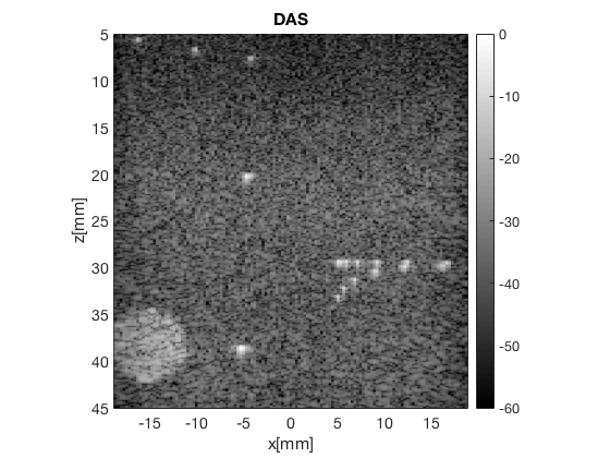
Define the DAS beamformer using coherent compounding of delayed data

das = postprocess.coherent_compounding();
das.input = delayed_b_data;
b_data_das = das.go();

b_data_das.plot([],'DAS');

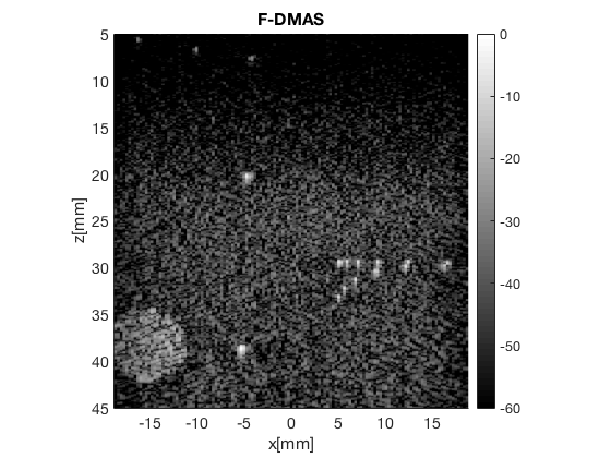
Create the DMAS image using the delay_multiply_and_sum postprocess

dmas = postprocess.delay_multiply_and_sum();
dmas.dimension = dimension.receive;
dmas.channel_data = channel_data;
dmas.input = delayed_b_data;
dmas.receive_apodization = delay.receive_apodization;

b_data_dmas=dmas.go();

% beamforming
b_data_dmas.plot(100,'F-DMAS');

Warning: Missing probe and apodization data; full aperture is assumed. 
Warning: If the result looks funky, you might need to tune the filter paramters
of DMAS using the filter_freqs property. Use the plot to check that everything
is OK. 

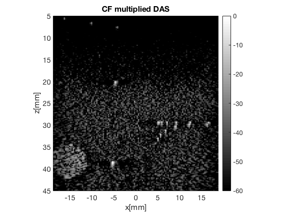
Calculate the coherence factor (CF) image

cf = postprocess.coherence_factor();
cf.dimension = dimension.receive();
cf.input = delayed_b_data;
b_data_CF_multiplied_DAS = cf.go();

b_data_CF_multiplied_DAS.plot(101,'CF multiplied DAS');

% Get just the CF "factor"
cfImg = cf.CF.get_image('none');

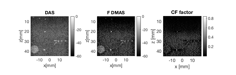
Plot all three images in same plot - Fig. 5

f3 = figure(3);clf
b_data_das.plot(subplot(1,3,1),'DAS'); % Display image
ax(1) = gca;
b_data_dmas.plot(subplot(1,3,2),'F DMAS'); % Display image
ax(2) = gca;
subplot(1,3,3)
imagesc(scan.x_axis*1e3,scan.z_axis*1e3,cfImg);colormap gray;title('CF factor');
xlabel('x [mm]');ylabel('z [mm]');
colorbar;axis('image')
set(gca,'FontSize',15);
ax(3) = gca;
linkaxes(ax);
set(gcf,'Position',[195   446   793   253]);

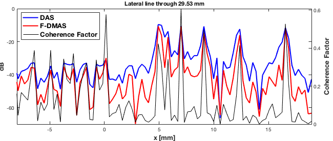
dmas_img = b_data_dmas.get_image();
das_img = b_data_das.get_image();
line_idx = find(b_data_dmas.scan.z_axis>=29.52e-3,1,'first');
x_axis=b_data_dmas.scan.x_axis;
pdmas=dmas_img(line_idx,:);
pdas=das_img(line_idx,:);
cfl=cfImg(line_idx,:);

% Plotting Fig. 6
figure('color','w','position',[244   164   650   276]);
subplot('position',[0.05 0.12 0.885 0.82])
[hAx,hLine1,hLine2] = plotyy([x_axis*1000, x_axis*1000],[pdas.', pdmas.'],x_axis*1000,cfl);
hLine1(1).LineWidth=2;hLine1(1).Color='b';
hLine1(2).LineWidth=2;hLine1(2).Color='r';
hLine2.Color='k';%hLine2.LineStyle='--';
hAx(1).YLim=[-70 0];hAx(1).XLim=[-8 max(x_axis*1000)];
hAx(2).YLim=[0 max(cfl)];hAx(2).XLim=[-8 max(x_axis*1000)];
hAx(1).YLabel.String='dB';hAx(1).YLabel.FontWeight='bold';
hAx(2).YLabel.String='Coherence Factor';hAx(2).YLabel.FontWeight='bold';
hAx(1).YLabel.FontSize=13;hAx(2).YLabel.FontSize=13;
hAx(1).XLabel.String='x [mm]';hAx(1).XLabel.FontWeight='bold';
hAx(1).XLabel.FontSize=13;
hAx(2).YColor=hAx(1).YColor;grid

title(sprintf('Lateral line through %.2f mm',...
                                  b_data_dmas.scan.z_axis(line_idx)*10^3));
h=legend('DAS','F-DMAS','Coherence Factor','location','northwest');grid
set(h,'fontsize',13,'fontweight','bold')

Published with MATLAB® R2018a